# Kaggle: Predict the occurrence of diabetes

This project presents a code/kernel used in a Kaggle competition promoted by [Data Science Academy](https://www.datascienceacademy.com.br/) in January of 2019.

The goal of the competition was to create a Machine Learning model to predict the occurrence of diabetes.

Data source: National Institute of Diabetes and Digestive and Kidney Diseases

Competition page: https://www.kaggle.com/c/competicao-dsa-machine-learning-jan-2019/

---

# Predict the occurrence of diabetes

Above the EDA is presented with the source code used to perform the data pre-processing, data transformation, and create the machine learning models.

## Exploratory Data Analysis

Data fields:
* num_gestacoes - Number of times pregnant
* glicose - Plasma glucose concentration in oral glucose tolerance test
* pressao_sanguinea - Diastolic blood pressure in mm Hg
* grossura_pele - Thickness of the triceps skinfold in mm
* insulina - Insulin (mu U / ml)
* bmi - Body mass index measured by weight in kg / (height in m) ^ 2
* indice_historico - Diabetes History Index (Pedigree Function)
* idade - Age in years
* classe - Class (0 - did not develop disease / 1 - developed disease)

### Loading the data


```python
# Importing packages
import numpy as np 
import pandas as pd 
import seaborn as sns
from scipy import stats
import matplotlib.pyplot as plt
import warnings
warnings.filterwarnings("ignore", category=FutureWarning)
%matplotlib inline

# Loading the data
data = pd.read_csv('data/dataset_treino.csv')
test_data = pd.read_csv('data/dataset_teste.csv')
data.head(5)
```




<div>
<style scoped>
    .dataframe tbody tr th:only-of-type {
        vertical-align: middle;
    }

    .dataframe tbody tr th {
        vertical-align: top;
    }

    .dataframe thead th {
        text-align: right;
    }
</style>
<table border="1" class="dataframe">
  <thead>
    <tr style="text-align: right;">
      <th></th>
      <th>id</th>
      <th>num_gestacoes</th>
      <th>glicose</th>
      <th>pressao_sanguinea</th>
      <th>grossura_pele</th>
      <th>insulina</th>
      <th>bmi</th>
      <th>indice_historico</th>
      <th>idade</th>
      <th>classe</th>
    </tr>
  </thead>
  <tbody>
    <tr>
      <th>0</th>
      <td>1</td>
      <td>6</td>
      <td>148</td>
      <td>72</td>
      <td>35</td>
      <td>0</td>
      <td>33.6</td>
      <td>0.627</td>
      <td>50</td>
      <td>1</td>
    </tr>
    <tr>
      <th>1</th>
      <td>2</td>
      <td>1</td>
      <td>85</td>
      <td>66</td>
      <td>29</td>
      <td>0</td>
      <td>26.6</td>
      <td>0.351</td>
      <td>31</td>
      <td>0</td>
    </tr>
    <tr>
      <th>2</th>
      <td>3</td>
      <td>8</td>
      <td>183</td>
      <td>64</td>
      <td>0</td>
      <td>0</td>
      <td>23.3</td>
      <td>0.672</td>
      <td>32</td>
      <td>1</td>
    </tr>
    <tr>
      <th>3</th>
      <td>4</td>
      <td>1</td>
      <td>89</td>
      <td>66</td>
      <td>23</td>
      <td>94</td>
      <td>28.1</td>
      <td>0.167</td>
      <td>21</td>
      <td>0</td>
    </tr>
    <tr>
      <th>4</th>
      <td>5</td>
      <td>0</td>
      <td>137</td>
      <td>40</td>
      <td>35</td>
      <td>168</td>
      <td>43.1</td>
      <td>2.288</td>
      <td>33</td>
      <td>1</td>
    </tr>
  </tbody>
</table>
</div>



### Data overview


```python
# General statistics
data.info()
```

    <class 'pandas.core.frame.DataFrame'>
    RangeIndex: 600 entries, 0 to 599
    Data columns (total 10 columns):
    id                   600 non-null int64
    num_gestacoes        600 non-null int64
    glicose              600 non-null int64
    pressao_sanguinea    600 non-null int64
    grossura_pele        600 non-null int64
    insulina             600 non-null int64
    bmi                  600 non-null float64
    indice_historico     600 non-null float64
    idade                600 non-null int64
    classe               600 non-null int64
    dtypes: float64(2), int64(8)
    memory usage: 47.0 KB


All 10 predictors variables (features) are quantitative (numerical) and we have 600 observations to build the prediction model.

The only qualitative column is the labels, where:

* 0 - do not have the disease
* 1 - have the disease


### Data Cleaning

#### Checking if there are missing values


```python
# If the result is False, there is no missing value
data.isnull().values.any()
```




    False



#### Computing statistics for each column


```python
data.describe()
```




<div>
<style scoped>
    .dataframe tbody tr th:only-of-type {
        vertical-align: middle;
    }

    .dataframe tbody tr th {
        vertical-align: top;
    }

    .dataframe thead th {
        text-align: right;
    }
</style>
<table border="1" class="dataframe">
  <thead>
    <tr style="text-align: right;">
      <th></th>
      <th>id</th>
      <th>num_gestacoes</th>
      <th>glicose</th>
      <th>pressao_sanguinea</th>
      <th>grossura_pele</th>
      <th>insulina</th>
      <th>bmi</th>
      <th>indice_historico</th>
      <th>idade</th>
      <th>classe</th>
    </tr>
  </thead>
  <tbody>
    <tr>
      <th>count</th>
      <td>600.000000</td>
      <td>600.000000</td>
      <td>600.000000</td>
      <td>600.000000</td>
      <td>600.000000</td>
      <td>600.000000</td>
      <td>600.000000</td>
      <td>600.000000</td>
      <td>600.000000</td>
      <td>600.000000</td>
    </tr>
    <tr>
      <th>mean</th>
      <td>300.500000</td>
      <td>3.820000</td>
      <td>120.135000</td>
      <td>68.681667</td>
      <td>20.558333</td>
      <td>79.528333</td>
      <td>31.905333</td>
      <td>0.481063</td>
      <td>33.278333</td>
      <td>0.346667</td>
    </tr>
    <tr>
      <th>std</th>
      <td>173.349358</td>
      <td>3.362009</td>
      <td>32.658246</td>
      <td>19.360226</td>
      <td>16.004588</td>
      <td>116.490583</td>
      <td>8.009638</td>
      <td>0.337284</td>
      <td>11.822315</td>
      <td>0.476306</td>
    </tr>
    <tr>
      <th>min</th>
      <td>1.000000</td>
      <td>0.000000</td>
      <td>0.000000</td>
      <td>0.000000</td>
      <td>0.000000</td>
      <td>0.000000</td>
      <td>0.000000</td>
      <td>0.078000</td>
      <td>21.000000</td>
      <td>0.000000</td>
    </tr>
    <tr>
      <th>25%</th>
      <td>150.750000</td>
      <td>1.000000</td>
      <td>99.000000</td>
      <td>64.000000</td>
      <td>0.000000</td>
      <td>0.000000</td>
      <td>27.075000</td>
      <td>0.248000</td>
      <td>24.000000</td>
      <td>0.000000</td>
    </tr>
    <tr>
      <th>50%</th>
      <td>300.500000</td>
      <td>3.000000</td>
      <td>116.000000</td>
      <td>70.000000</td>
      <td>23.000000</td>
      <td>36.500000</td>
      <td>32.000000</td>
      <td>0.384000</td>
      <td>29.000000</td>
      <td>0.000000</td>
    </tr>
    <tr>
      <th>75%</th>
      <td>450.250000</td>
      <td>6.000000</td>
      <td>140.000000</td>
      <td>80.000000</td>
      <td>32.000000</td>
      <td>122.750000</td>
      <td>36.525000</td>
      <td>0.647000</td>
      <td>40.000000</td>
      <td>1.000000</td>
    </tr>
    <tr>
      <th>max</th>
      <td>600.000000</td>
      <td>17.000000</td>
      <td>198.000000</td>
      <td>122.000000</td>
      <td>99.000000</td>
      <td>846.000000</td>
      <td>67.100000</td>
      <td>2.420000</td>
      <td>81.000000</td>
      <td>1.000000</td>
    </tr>
  </tbody>
</table>
</div>



From the table above, we can see the zero values in almost all columns.
For some of these columns, zero makes sense, like for Pregnancies and Outcome. But for some of the others, like BloodPressure or BMI, zero definitely doesn't make sense. 

After read some papers about the variables in the dataset, I see that some columns can have a value very close to zero (e.g. *grossura_pele*), but others can't have a zero value. 

The columns can not have a zero value. 
* glicose
* pressao_sanguinea
* bmi

Let's see the number of the occurrences of zero values for all columns:


```python
# Compute the number of occurrences of a zero value 
features = ['num_gestacoes', 'glicose', 'pressao_sanguinea', 'grossura_pele', 'insulina', 'bmi', 'indice_historico', 'idade']
for c in features:
    counter = len(data[data[c] == 0])    
    print('{} - {}'.format(c, counter))    
```

    num_gestacoes - 93
    glicose - 5
    pressao_sanguinea - 28
    grossura_pele - 175
    insulina - 289
    bmi - 9
    indice_historico - 0
    idade - 0


We can also see that column *insulina* has 289 values, which correspond to 48% of the training data.

Let's remove these observations from the selected columns.


```python
# Removing observations with zero value
data_cleaned = data.copy()   
for c in ['glicose', 'pressao_sanguinea', 'bmi']:
    data_cleaned = data_cleaned[data_cleaned[c] != 0]

data_cleaned.shape
```




    (564, 10)



The final number of observations was 564. 

Let's see the compute some statistics again:


```python
data_cleaned.describe()
```




<div>
<style scoped>
    .dataframe tbody tr th:only-of-type {
        vertical-align: middle;
    }

    .dataframe tbody tr th {
        vertical-align: top;
    }

    .dataframe thead th {
        text-align: right;
    }
</style>
<table border="1" class="dataframe">
  <thead>
    <tr style="text-align: right;">
      <th></th>
      <th>id</th>
      <th>num_gestacoes</th>
      <th>glicose</th>
      <th>pressao_sanguinea</th>
      <th>grossura_pele</th>
      <th>insulina</th>
      <th>bmi</th>
      <th>indice_historico</th>
      <th>idade</th>
      <th>classe</th>
    </tr>
  </thead>
  <tbody>
    <tr>
      <th>count</th>
      <td>564.000000</td>
      <td>564.000000</td>
      <td>564.000000</td>
      <td>564.000000</td>
      <td>564.000000</td>
      <td>564.000000</td>
      <td>564.000000</td>
      <td>564.000000</td>
      <td>564.000000</td>
      <td>564.000000</td>
    </tr>
    <tr>
      <th>mean</th>
      <td>300.664894</td>
      <td>3.845745</td>
      <td>121.354610</td>
      <td>72.049645</td>
      <td>21.432624</td>
      <td>84.406028</td>
      <td>32.367199</td>
      <td>0.483294</td>
      <td>33.448582</td>
      <td>0.340426</td>
    </tr>
    <tr>
      <th>std</th>
      <td>173.410435</td>
      <td>3.349287</td>
      <td>31.130992</td>
      <td>12.261552</td>
      <td>15.809953</td>
      <td>118.432015</td>
      <td>6.974710</td>
      <td>0.337668</td>
      <td>11.868844</td>
      <td>0.474273</td>
    </tr>
    <tr>
      <th>min</th>
      <td>1.000000</td>
      <td>0.000000</td>
      <td>44.000000</td>
      <td>24.000000</td>
      <td>0.000000</td>
      <td>0.000000</td>
      <td>18.200000</td>
      <td>0.078000</td>
      <td>21.000000</td>
      <td>0.000000</td>
    </tr>
    <tr>
      <th>25%</th>
      <td>150.750000</td>
      <td>1.000000</td>
      <td>99.000000</td>
      <td>64.000000</td>
      <td>0.000000</td>
      <td>0.000000</td>
      <td>27.300000</td>
      <td>0.250500</td>
      <td>24.000000</td>
      <td>0.000000</td>
    </tr>
    <tr>
      <th>50%</th>
      <td>298.500000</td>
      <td>3.000000</td>
      <td>116.000000</td>
      <td>72.000000</td>
      <td>23.500000</td>
      <td>49.000000</td>
      <td>32.000000</td>
      <td>0.389000</td>
      <td>29.000000</td>
      <td>0.000000</td>
    </tr>
    <tr>
      <th>75%</th>
      <td>450.250000</td>
      <td>6.000000</td>
      <td>141.250000</td>
      <td>80.000000</td>
      <td>33.000000</td>
      <td>130.000000</td>
      <td>36.600000</td>
      <td>0.648250</td>
      <td>41.000000</td>
      <td>1.000000</td>
    </tr>
    <tr>
      <th>max</th>
      <td>600.000000</td>
      <td>17.000000</td>
      <td>198.000000</td>
      <td>122.000000</td>
      <td>99.000000</td>
      <td>846.000000</td>
      <td>67.100000</td>
      <td>2.420000</td>
      <td>81.000000</td>
      <td>1.000000</td>
    </tr>
  </tbody>
</table>
</div>



#### Checking outliers

Let's check if there are outliers in the data.

First, we'll use a set of boxplots, one for each column.


```python
fig, axes = plt.subplots(2,4, figsize=(20,8))

x,y = 0,0
for i, column in enumerate(data_cleaned.columns[1:-1]):    
    sns.boxplot(x=data_cleaned[column], ax=axes[x,y])
    if i < 3:
        y += 1
    elif i == 3: 
        x = 1
        y = 0
    else:
        y += 1
```

![output_18_0.png](https://cdn.hashnode.com/res/hashnode/image/upload/v1628594681273/utEdnFi_Ng.png)


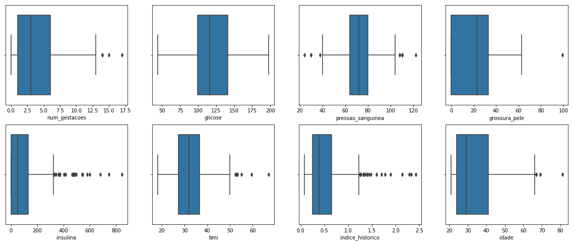
We can see some possible outliers for almost all columns (separated points in the plots).

The outliers can either be a mistake or just variance. For now, let's consider all of them as mistakes.

To remove these outliers we can use Z-Score or IQR (Interquartile Range).

The Z-score is the signed number of standard deviations by which the value of an observation or data point is above the mean value of what is being observed or measured. Z-score is finding the distribution of data where the mean is 0 and the standard deviation is 1. While calculating the Z-score we re-scale and center the data and look for data points that are too far from zero. These data points which are way too far from zero will be treated as outliers. In most of the cases, a threshold of 3 or -3 is used i.e if the Z-score value is greater than or less than 3 or -3 respectively, that data point will be identified as outliers.

Let's use the Z-score function defined in the Scipy library to detect the outliers:


```python
# Compute the Z-Score for each column

print(data_cleaned.shape)

z = np.abs(stats.zscore(data_cleaned))    
data_cleaned = data_cleaned[(z < 3).all(axis=1)]   

print(data_cleaned.shape)    
```

    (564, 10)
    (531, 10)


Using Z-Score, 33 observations were removed.

Let's see the boxplots again:


```python
fig, axes = plt.subplots(2,4, figsize=(20,8))

x,y = 0,0
for i, column in enumerate(data_cleaned.columns[1:-1]):    
    sns.boxplot(x=data_cleaned[column], ax=axes[x,y], palette="Set2")
    if i < 3:
        y += 1
    elif i == 3: 
        x = 1
        y = 0
    else:
        y += 1
```

![output_22_0.png](https://cdn.hashnode.com/res/hashnode/image/upload/v1628594697160/jDIgcu3hk.png)

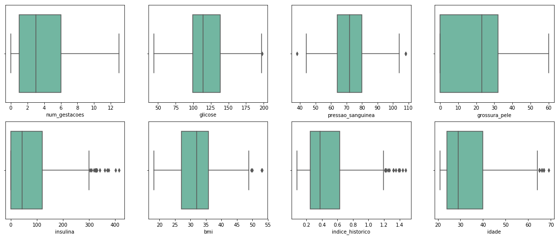
The data was much cleaner now. Still, there are some points in the boxplots, but some of them are not outliers, like the *insulina* values higher than 400, which is acceptable in people with diabetes. 

#### Checking the balance of the dataset

Let's checking the distribuitions of examples for each label:


```python
data_cleaned.classe.value_counts().plot(kind='bar');
```

![output_25_0.png](https://cdn.hashnode.com/res/hashnode/image/upload/v1628594716223/hEPyVxt_P.png)


```python
data_cleaned.classe.value_counts(normalize=True)
```




    0    0.676083
    1    0.323917
    Name: classe, dtype: float64



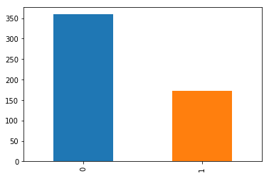
From the figure above, we see most of our examples are of people that do not have the disease. More specifically, 67% of the data are for healthy people.

As the dataset is unbalanced, let's use some methods to reduce the unbalance of the classes.

I use the over-sampling SMOTE method.
SMOTE (Synthetic Minority Oversampling Technique) consists of synthesizing elements for the minority class, based on those that already exist. It works randomly picking a point from the minority class and computing the k-nearest neighbors for this point. The synthetic points are added between the chosen point and its neighbors.



```python
from imblearn.over_sampling import SMOTE

# Select the columns with features
features = ['num_gestacoes', 'glicose', 'pressao_sanguinea', 'grossura_pele', 'insulina', 'bmi', 'indice_historico', 'idade']
X = data_cleaned[features]
# Select the columns with labels
Y = data_cleaned['classe']

smote = SMOTE(sampling_strategy=1.0, k_neighbors=4)
X_sm, y_sm = smote.fit_sample(X, Y)

print(X_sm.shape[0] - X.shape[0], 'new random picked points')
data_cleaned_oversampled = pd.DataFrame(X_sm, columns=data.columns[1:-1])
data_cleaned_oversampled['classe'] = y_sm
data_cleaned_oversampled['id'] = range(1,len(y_sm)+1)

for c in ['num_gestacoes', 'glicose', 'pressao_sanguinea', 'grossura_pele', 'insulina', 'idade']:
    data_cleaned_oversampled[c] = data_cleaned_oversampled[c].apply(lambda x: int(x))

data_cleaned_oversampled.classe.value_counts().plot(kind='bar');
```

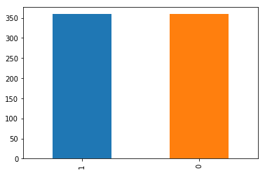
    187 new random picked points


![output_28_1.png](https://cdn.hashnode.com/res/hashnode/image/upload/v1628594733879/O1UebUb-iH.png)


## Training the Model

Now that data is cleaned, let's use a machine learning model to predict whether or not a person has diabetes.

The metric used in this competition is the **accuracy score**.

### Using Decision Tree


```python
from sklearn.model_selection import train_test_split
from sklearn.metrics import accuracy_score
from sklearn.metrics import confusion_matrix
from sklearn import tree

# Select the columns with features
features = ['num_gestacoes', 'glicose', 'pressao_sanguinea', 'grossura_pele', 'insulina', 'bmi', 'indice_historico', 'idade']
X = data_cleaned_oversampled[features]
# Select the columns with labels
Y = data_cleaned_oversampled['classe']

# Perform the training and test 100 times with different seeds and compute the mean accuracy.
# Save results
acurrances = []
for i in range(100):    
    # Spliting Dataset into Test and Train
    X_train, X_test, y_train, y_test = train_test_split(X, Y, test_size=0.3, random_state=i)

    # Create and train the model
    clf = tree.DecisionTreeClassifier(criterion = 'entropy', random_state=i, max_depth=4)
    clf.fit(X_train,y_train)

    # Performing predictions with test dataset
    y_pred = clf.predict(X_test)
    # Computing accuracy    
    acurrances.append(accuracy_score(y_test, y_pred)*100)

print('Accuracy is ', np.mean(acurrances))
```

    Accuracy is  73.35648148148148


### Using Logistic Regression (LR)



```python
from sklearn.linear_model import LogisticRegression
from sklearn.metrics import classification_report, confusion_matrix

# Select the columns with features
features = ['num_gestacoes', 'glicose', 'pressao_sanguinea', 'grossura_pele', 'insulina', 'bmi', 'indice_historico', 'idade']

# For the LR the oversampled database decreased the model accuracy, so I choose do not to use it.
X = data_cleaned[features]
# Select the columns with labels
Y = data_cleaned['classe']

# Perform the training and test 100 times with different seeds and compute the mean accuracy.
# Save results
acurrances = []
for i in range(100):    
    # Spliting the data
    X_train, X_test, y_train, y_test = train_test_split(X, Y, test_size=0.3, random_state=i)
    LR_model=LogisticRegression(class_weight={1:1.15})
    LR_model.fit(X_train,y_train)

    # Testing
    y_pred=LR_model.predict(X_test)
    acurrances.append(accuracy_score(y_test, y_pred)*100)
    
    # Print only the last
    if i == 99:
        pass
        #print(classification_report(y_test,y_pred))
        #print(confusion_matrix(y_true=y_test, y_pred=y_pred))

print('Accuracy is ', np.mean(acurrances))
```

    Accuracy is  76.725


### Feature selection

The large number of zero values in the *grossura_pele* and *insulina* are impairing the performance of the model.
So, as insulin is an important parameter in the evaluation of diabetes let's replace the zeros values by the mean
for both columns.

As the Logistic Regression (LR) performs better than the Decision Tree. I'll use only LR from now.


```python
# Replacing the zeros by the mean
data_cleaned_no_zeros = data_cleaned.copy()

for c in ['grossura_pele', 'insulina']:    
    feature_avg =data_cleaned[data_cleaned[c]>0][[c]].mean()
    data_cleaned[c]=np.where(data_cleaned[[c]]!=0,data_cleaned[[c]],feature_avg)
```


```python
# Select the columns with features
features = ['num_gestacoes', 'glicose', 'pressao_sanguinea', 'grossura_pele', 'insulina', 'bmi', 'indice_historico', 'idade']
X = data_cleaned_no_zeros[features]
# Select the columns with labels
Y = data_cleaned_no_zeros['classe']

# Perform the training and test 100 times with different seeds and compute the mean accuracy score.
# Save results
acurrances = []
for i in range(100):    
    # Spliting the data
    X_train, X_test, y_train, y_test = train_test_split(X, Y, test_size=0.3, random_state=i)
    LR_model=LogisticRegression(class_weight={1:1.1})
    LR_model.fit(X_train,y_train)

    # Testing
    y_pred=LR_model.predict(X_test)
    acurrances.append(accuracy_score(y_test, y_pred)*100)
    
    # Print only the last
    if i == 99:
        print(classification_report(y_test,y_pred))
        print(confusion_matrix(y_true=y_test, y_pred=y_pred))

print('Accuracy is ', np.mean(acurrances))

```

                  precision    recall  f1-score   support
    
               0       0.83      0.91      0.87       110
               1       0.75      0.60      0.67        50
    
       micro avg       0.81      0.81      0.81       160
       macro avg       0.79      0.75      0.77       160
    weighted avg       0.81      0.81      0.81       160
    
    [[100  10]
     [ 20  30]]
    Accuracy is  76.5625


The performance decrease when I replace the zeros values by the mean for *grossura_pele* and *insulina* columns.



## Performing the Final Prediction

For the final model, I choose to use LR with the cleaned dataset.


```python
# Create and train the model with all data
model=LogisticRegression(class_weight={1:1.1})
model.fit(data_cleaned[features],data_cleaned['classe'])

# Get the kaggle test data
X_test = test_data[features]
# Make the prediction 
prediction = model.predict(X_test)

# Add the predictions to the dataframe 
test_data['classe'] = prediction

# Create the submission file
test_data.loc[:,['id', 'classe']].to_csv('submission.csv', encoding='utf-8', index=False)
```


---
# Source code

The solution is also available at Github.

[![GitHub](/github.jpg)](https://github.com/cpatrickalves/kaggle-diabetes-prediction)

#### How to use

* You will need Python 3.5+ to run the code.
* Python can be downloaded [here](https://www.python.org/downloads/).
* You have to install some Python packages, in command prompt/Terminal: `pip install jupyter-lab scikit-learn pandas seaborn matplotlib`
* Once you have installed the required packages, just clone/download this project:
`git clone https://github.com/cpatrickalves/kaggle-diabetes-prediction`

* Access the project folder in command prompt/Terminal and run the following command:
`jupyter-lab`

* Then open the **kernel** file.