This project presents a code/kernel used in a Kaggle competition promoted by Data Science Academy in September of 2019.

The goal of the competition was to create a Machine Learning model to help a robot to classify the floor surface on which it is using data collected by Inertial Measurement Units (IMU) sensors.

About the project

The data used in this competition was collected by the Tampere University Signal Processing Department in Finland. Data collection was performed with a small mobile robot equipped with IMU sensors on different floor surfaces at the university premises. The task is to predict which of the nine floor types (carpet, tiles, concrete, etc.) the robot is using sensor data such as acceleration and velocity. The success of this competition will help improve the navigation of autonomous robots on many different surfaces.

Competition page: https://www.kaggle.com/c/competicao-dsa-machine-learning-sep-2019

The evaluation metric for this competition was the Multiclass Accuracy, which is simply the average rating number with the correct label.

In this competition, my best score was 62.2% and I've got position 26 on the leaderboard.

Source code

The solution is also available at Github.

How to use

You will need Python 3.5+ to run the code.
Python can be downloaded here.
You have to install some Python packages, in command prompt/Terminal: pip install -r requirements.txt
Once you have installed the required packages, just clone/download this project: git clone https://github.com/cpatrickalves/kaggle-floor-surface-classification
Access the project folder in command prompt/Terminal and run the following command: jupyter-lab

The datasets are available on the competition's pages.

Files description:

X_treino.csv - contains the training dataset with 487,680 rows and 13 columns.
X_teste.csv - contains the test dataset with 488,448 rows and 13 columns.
y_treino.csv - the surfaces for the training set.
sample_submission.csv - a sample submission file in the correct format.

Classifying the type of flooring surface

In the following lines I've described in more detail the solution built.

Exploratory Data Analysis

The sensor data collected includes accelerometer data, gyroscope data (angular rate) and internally estimated orientation. Specifically:

Orientation: 4 attitude quaternion (a mathematical notation used to represent orientations and rotations in a 3D space) channels, 3 for vector part and one for the scalar part;
Angular rate: 3 channels, corresponding to the 3 IMU coordinate axes X, Y, and Z;
Acceleration: 3 channels, specific force corresponding to 3 IMU coordinate axes X, Y, and Z.

Each data point includes the measures described above of orientation, velocity, and acceleration, resulting in a feature vector of length 10 for each point.

There are 128 measurements per time series plus three identification columns:

row_id: The ID for the row.
series_id: a number that identifies the measurement series. It is also the foreign key to y_train and sample_submission.
measurement_number: measurement number within the series.

Loading the data

# If you will use tqdm
#!pip install ipywidgets
#!jupyter nbextension enable --py widgetsnbextension
#!pip install -r requirements.txt

import pandas as pd
import matplotlib.pyplot as plt
import seaborn as sns
import numpy as np
from tqdm import tqdm_notebook as tqdm
%matplotlib inline

# Folder with datasets
data_folder = "data/"

# Running on kaggle?
kaggle = False

if kaggle:
    data_folder = "../input/"

# Load the data for training ML models
xtrain = pd.read_csv(data_folder + "X_treino.csv")
ytrain = pd.read_csv(data_folder + "y_treino.csv") # Target
train_data = pd.merge(xtrain, ytrain, how = "left", on = "series_id")

#Load the Test dataset to predict the results (used for submission)
xtest = pd.read_csv(data_folder + "X_teste.csv")
test_data = xtest

# Submission data
submission = pd.read_csv(data_folder + "sample_submission.csv")

# Showing the number of samples and columns for each dataset
print(train_data.shape)
print(test_data.shape)

(487680, 15)
(488448, 13)

train_data.head()

	row_id	series_id	measurement_number	orientation_X	orientation_Y	orientation_Z	orientation_W	angular_velocity_X	angular_velocity_Y	angular_velocity_Z	linear_acceleration_X	linear_acceleration_Y	linear_acceleration_Z	group_id	surface
0	0_0	0	0	-0.75853	-0.63435	-0.10488	-0.10597	0.10765	0.017561	0.00076741	-0.74857	2.103	-9.7532	13	fine_concrete
1	0_1	0	1	-0.75853	-0.63434	-0.1049	-0.106	0.067851	0.029939	0.0033855	0.33995	1.5064	-9.4128	13	fine_concrete
2	0_2	0	2	-0.75853	-0.63435	-0.10492	-0.10597	0.0072747	0.028934	-0.0059783	-0.26429	1.5922	-8.7267	13	fine_concrete
3	0_3	0	3	-0.75852	-0.63436	-0.10495	-0.10597	-0.013053	0.019448	-0.0089735	0.42684	1.0993	-10.096	13	fine_concrete
4	0_4	0	4	-0.75852	-0.63435	-0.10495	-0.10596	0.0051349	0.0076517	0.0052452	-0.50969	1.4689	-10.441	13	fine_concrete

Frequency Distribution

# Check unique values
train_count_series = len(train_data.series_id.unique())
test_count_series = len(test_data.series_id.unique())
train_freq_distribution_surfaces = train_data.surface.value_counts()

print(f"Number of time series in train dataset: {train_count_series}")
print(f"Number of time series in test dataset: {test_count_series}\n")

print(f"Surfaces frequency distribution in train dataset:\n{train_freq_distribution_surfaces}")
train_freq_distribution_surfaces.plot(kind="barh", figsize=(10,5))
plt.title("Sample distribution by class")
plt.ylabel("Number of time series")
plt.show()

Number of time series in train dataset: 3810
Number of time series in test dataset: 3816

Surfaces frequency distribution in train dataset:
concrete                  99712
soft_pvc                  93696
wood                      77696
tiled                     65792
fine_concrete             46464
hard_tiles_large_space    39424
soft_tiles                38016
carpet                    24192
hard_tiles                 2688
Name: surface, dtype: int64

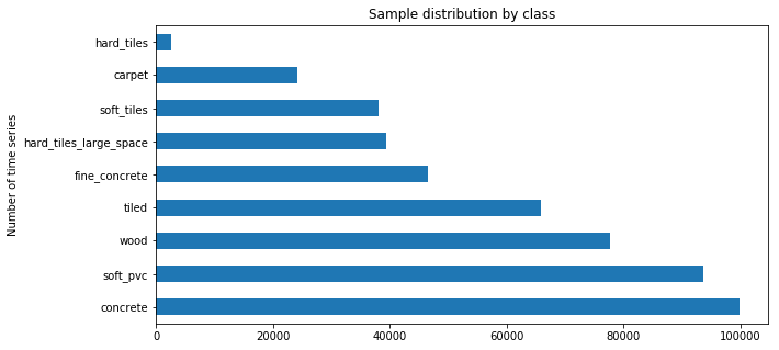
So, the train data set contains 3810 labeled time-series samples, with the corresponding surface type annotation.

Most of the samples are for the concrete surface. The hard_tiles has only 2688 samples, this may be insufficient to build a robust model for this type of surface.

Furthermore, the classes are not balanced so we need to be careful because a simple accuracy score is not enough to evaluate the model performance.

Frequency distribution for each column

plt.subplots_adjust(top=0.8)
for i, col in enumerate(xtrain.columns[3:]):
    g = sns.FacetGrid(train_data, col="surface", col_wrap=5, height=3, aspect=1.1)
    g = g.map(sns.distplot, col)
    g.fig.suptitle(col, y=1.09, fontsize=23)

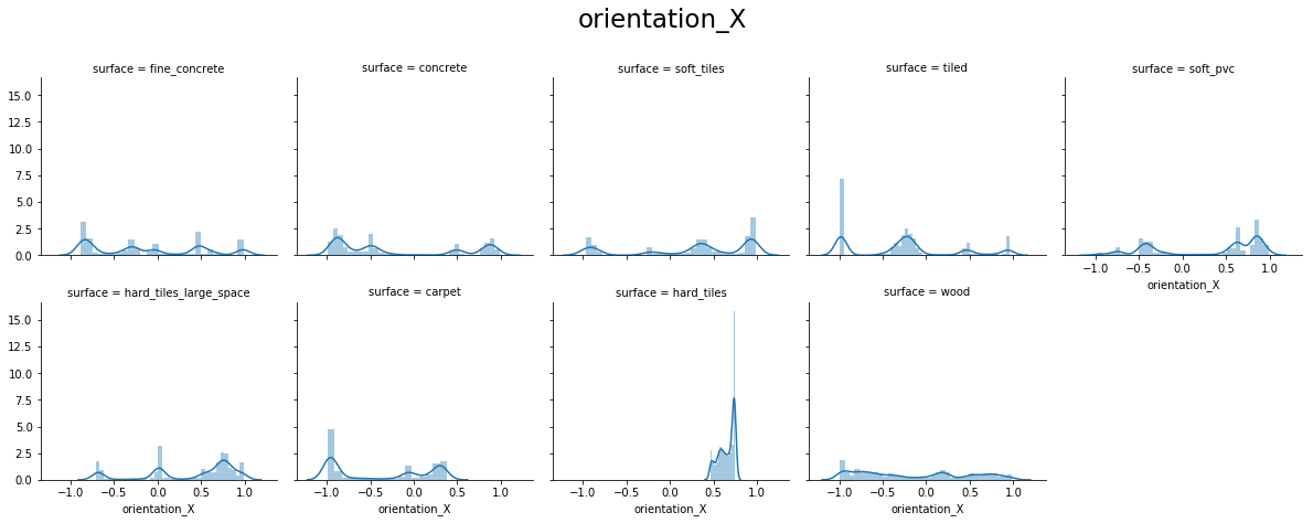
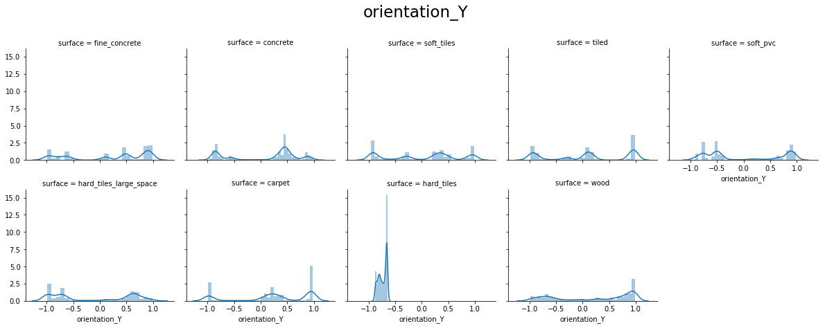
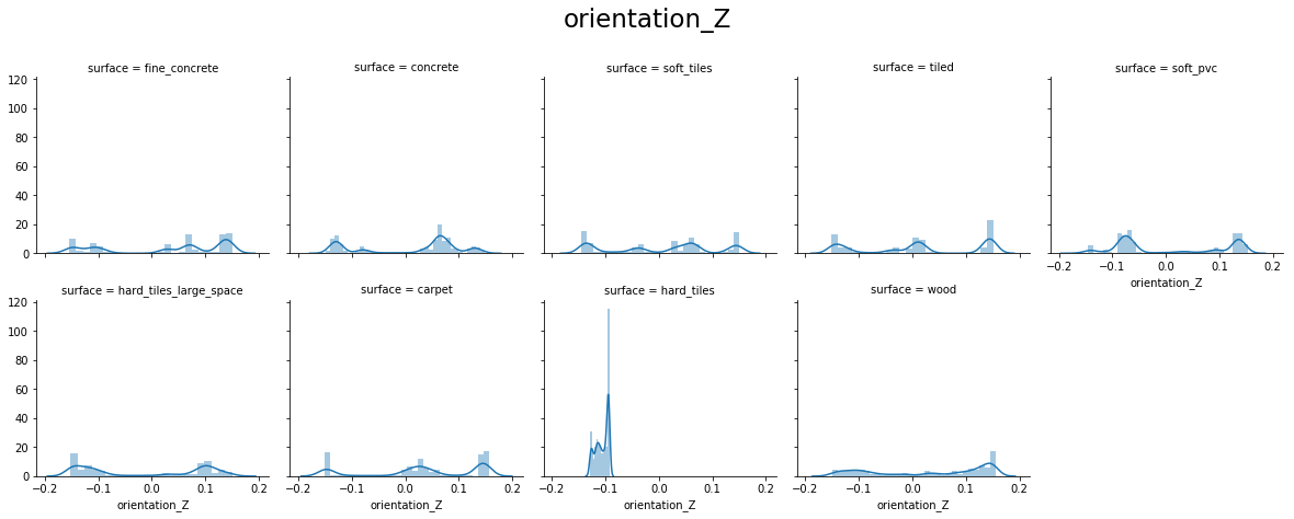
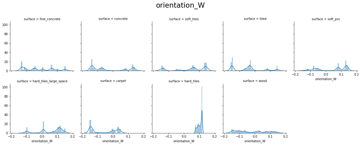
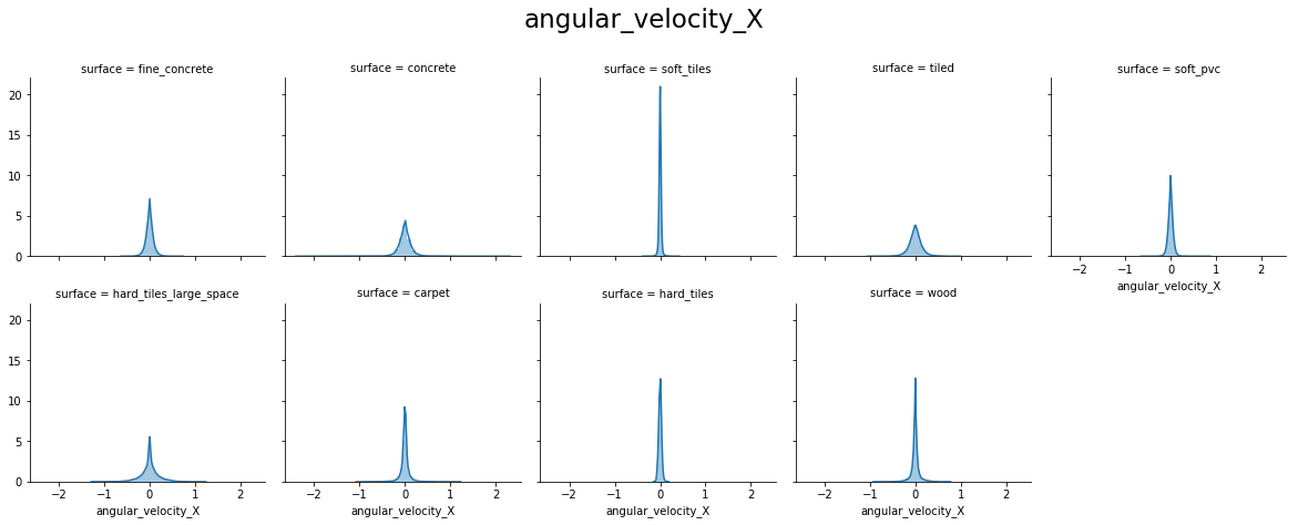
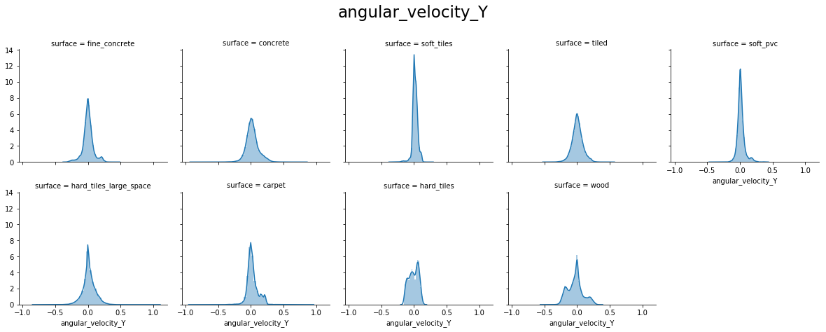
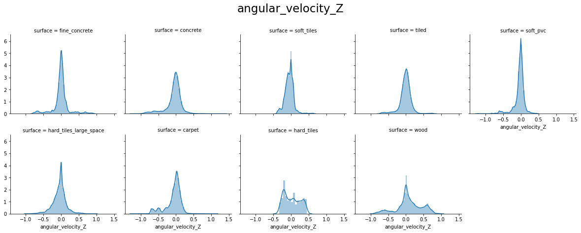
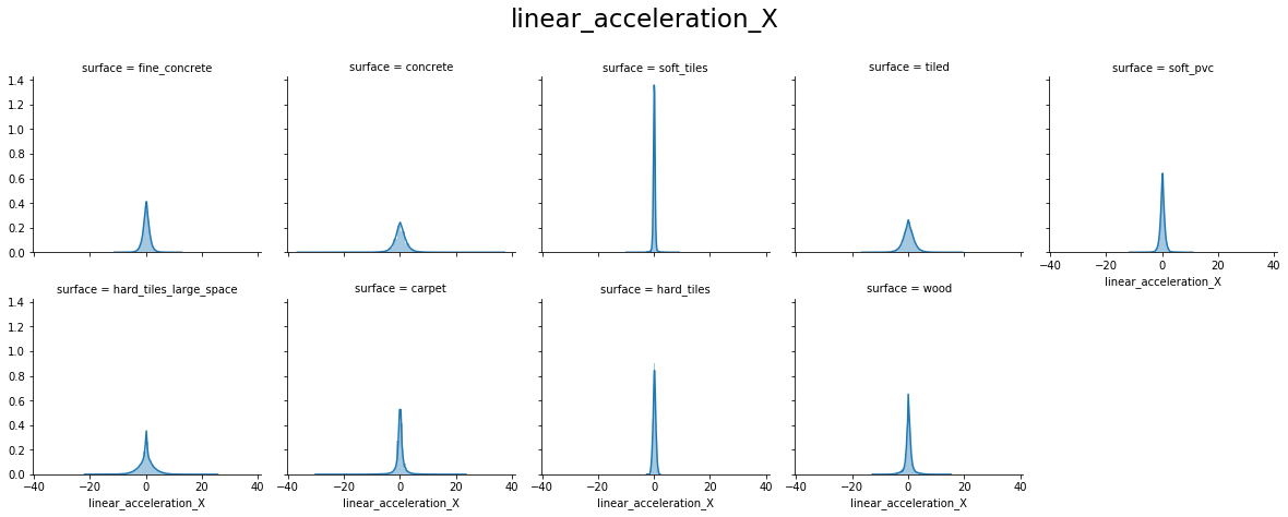
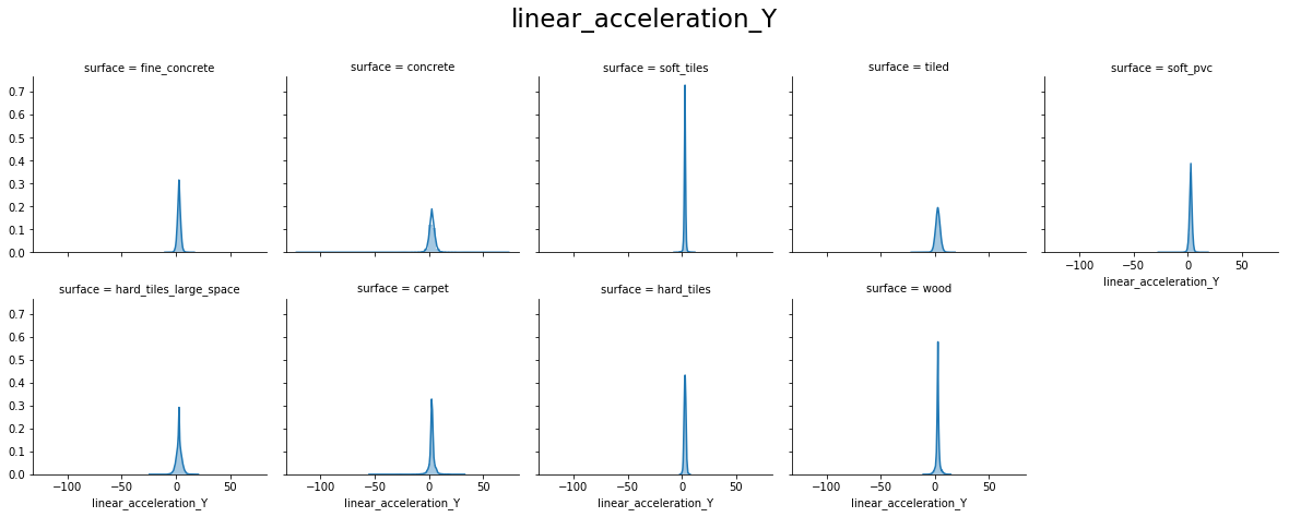
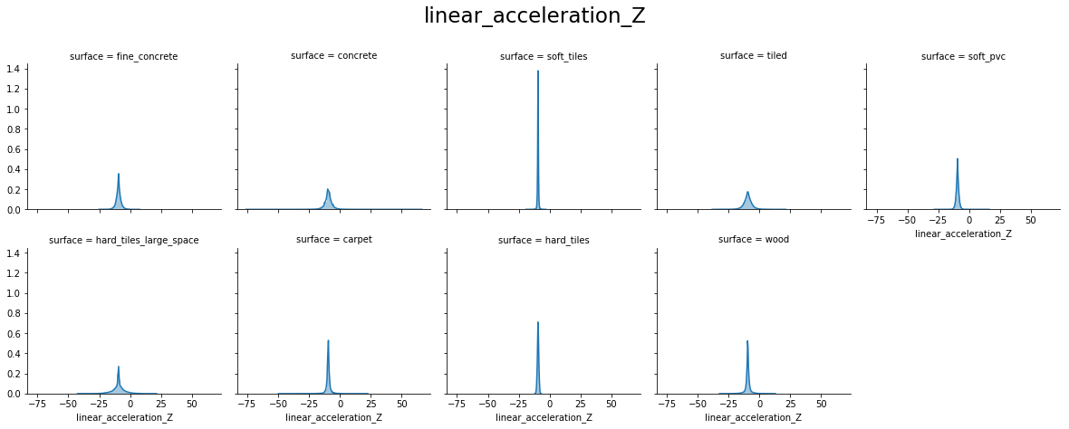
From the above plots, we can see that:

orientation X and orientation Y have values around -1.0 to 1.0
orientation Z and orientation W have values around -0.15 to 0.15
For orientation X, Y, Z, and W hard_tiles have different distributions as compared to others.
angular_velocity_x forms a perfect Normal distribution
angular_velocity_y and angular_velocity_z have distributions close to a Normal for most surfaces, excepts for hard_tiles, carpet and wood.
linear_acceleration_X, linear_acceleration_Y and linear_acceleration_Z forms a Normal distribution for all surfaces.

Feature Engineering

To build the ML model we'll convert each time series value to the following metrics:

Mean
Standard Deviation
Min and Max values
Kurtosis Coefficient
Skewness Coefficient

# Function that performs all data transformation and pre-processing
def data_preprocessing(df, labeled=False):

    # New dataframe that will saves the tranformed data
    X = pd.DataFrame()

    # This list will save the type of surface for each series ID
    Y = []

    # The selected attributes used in training
    selected_attributes = ['orientation_X', 'orientation_Y', 'orientation_Z', 'orientation_W',
                           'angular_velocity_X', 'angular_velocity_Y', 'angular_velocity_Z', 'linear_acceleration_X',
                           'linear_acceleration_Y', 'linear_acceleration_Z']

    # The total number of series in training data
    total_test_series = len(df.series_id.unique())

    for series in tqdm(range(total_test_series)):
    #for series in range(total_test_series):

        # Filter the series id in the DataFrame
        _filter = (df.series_id == series)

        # If data with labels
        if labeled:
            # Saves the type of surface (label) for each series ID
            Y.append((df.loc[_filter, 'surface']).values[0])

        # Compute new values for each attribute
        for attr in selected_attributes:

            # Compute a new attribute for each series and save in the X DataFrame
            X.loc[series, attr + '_mean'] = df.loc[_filter, attr].mean()
            X.loc[series, attr + '_std'] = df.loc[_filter, attr].std()
            X.loc[series, attr + '_min'] = df.loc[_filter, attr].min()
            X.loc[series, attr + '_max'] = df.loc[_filter, attr].max()
            X.loc[series, attr + '_kur'] = df.loc[_filter, attr].kurtosis()
            X.loc[series, attr + '_skew'] = df.loc[_filter,attr].skew()


    return X,Y

# Apply the Pre-Processing to train data
X_train, Y_train = data_preprocessing(train_data, labeled=True)

# Here is the result DataFrame
X_train.head()

	orientation_X_mean	orientation_X_std	orientation_X_min	orientation_X_max	orientation_X_kur	orientation_X_skew	orientation_Y_mean	orientation_Y_std	orientation_Y_min	orientation_Y_max	orientation_Y_kur	orientation_Y_skew	orientation_Z_mean	orientation_Z_std	orientation_Z_min	orientation_Z_max	orientation_Z_kur	orientation_Z_skew	orientation_W_mean	orientation_W_std	orientation_W_min	orientation_W_max	orientation_W_kur	orientation_W_skew	angular_velocity_X_mean	angular_velocity_X_std	angular_velocity_X_min	angular_velocity_X_max	angular_velocity_X_kur	angular_velocity_X_skew	angular_velocity_Y_mean	angular_velocity_Y_std	angular_velocity_Y_min	angular_velocity_Y_max	angular_velocity_Y_kur	angular_velocity_Y_skew	angular_velocity_Z_mean	angular_velocity_Z_std	angular_velocity_Z_min	angular_velocity_Z_max	angular_velocity_Z_kur	angular_velocity_Z_skew	linear_acceleration_X_mean	linear_acceleration_X_std	linear_acceleration_X_min	linear_acceleration_X_max	linear_acceleration_X_kur	linear_acceleration_X_skew	linear_acceleration_Y_mean	linear_acceleration_Y_std	linear_acceleration_Y_min	linear_acceleration_Y_max	linear_acceleration_Y_kur	linear_acceleration_Y_skew	linear_acceleration_Z_mean	linear_acceleration_Z_std	linear_acceleration_Z_min	linear_acceleration_Z_max	linear_acceleration_Z_kur	linear_acceleration_Z_skew
0	-0.758666	0.000362699	-0.75953	-0.75822	-0.646196	-0.659082	-0.634008	0.000471151	-0.63456	-0.63306	-1.18587	0.603197	-0.105474	0.0004318	-0.10614	-0.10461	-1.2401	0.193309	-0.10647	0.000389266	-0.10705	-0.10559	-0.8543	0.441564	-0.00248068	0.0528002	-0.16041	0.10765	0.238451	-0.342643	-0.00330603	0.0315441	-0.079404	0.072698	-0.587032	0.0163959	0.00753165	0.0171275	-0.030181	0.05172	-0.441086	0.126373	0.263418	0.911175	-1.8644	2.8538	-0.3927	0.132684	2.98419	1.38779	0.075417	5.3864	-1.07535	-0.364964	-9.32039	1.09504	-12.512	-6.2681	0.532135	0.0673912
1	-0.958606	0.000151349	-0.95896	-0.95837	-0.642996	-0.397289	0.241867	0.000498771	0.24074	0.2427	-0.536113	-0.422565	0.0316503	0.000508249	0.030504	0.032341	-0.742008	-0.51718	-0.146876	0.000521176	-0.14809	-0.14587	-0.76241	-0.169549	0.00460477	0.092309	-0.2548	0.28342	0.303844	-0.136062	-0.00775678	0.0465231	-0.13433	0.11208	0.757283	-0.246493	0.00620628	0.067533	-0.12161	0.12915	-1.23483	0.00470172	0.121867	1.10595	-3.1934	5.1002	3.17784	0.759101	2.76819	1.86446	-2.1492	6.685	-0.575238	-0.183139	-9.3889	2.12307	-16.928	-2.7449	1.3568	-0.126848
2	-0.512057	0.00137747	-0.51434	-0.50944	-1.05258	0.151971	-0.846171	0.000785087	-0.84779	-0.8449	-1.08213	-0.161786	-0.129371	0.000540564	-0.1303	-0.12852	-1.31011	-0.0344055	-0.0710819	0.000278231	-0.071535	-0.070378	-0.707431	0.511039	0.00264566	0.0601675	-0.15271	0.14192	-0.55882	0.205228	-0.00923168	0.0355304	-0.10781	0.091946	0.460044	-0.077528	0.0279892	0.0218657	-0.015697	0.08873	-0.52209	0.0691234	0.149711	0.756138	-2.593	1.8533	0.670531	-0.480996	2.88674	1.76979	-1.254	6.2105	-0.584675	-0.266815	-9.39578	1.14027	-12.499	-5.7442	0.446304	0.0858766
3	-0.939169	0.000227324	-0.93968	-0.93884	-1.07809	-0.0961058	0.31014	0.00045304	0.30943	0.31147	1.54041	1.23098	0.038955	0.00044918	0.037922	0.039799	-0.640886	0.09768	-0.142319	0.00137111	-0.14437	-0.13934	-1.19738	0.175628	0.000623955	0.179544	-0.40152	0.51913	0.0789898	-0.00357532	-0.00280411	0.0466998	-0.16815	0.13578	1.19154	-0.320948	0.00788664	0.0322652	-0.073414	0.085345	0.0328897	-0.272105	0.201791	1.47202	-3.7934	4.2032	0.177944	-0.210587	2.65792	4.20141	-5.8251	11.743	-0.900409	-0.11738	-9.45116	3.47853	-19.845	-0.5591	0.6705	-0.210103
4	-0.891301	0.00295532	-0.89689	-0.88673	-1.16594	-0.2267	0.428144	0.00616534	0.41646	0.4374	-1.1399	-0.242538	0.0600564	0.000985321	0.058247	0.061771	-1.45927	-0.0923971	-0.13646	0.000541113	-0.13732	-0.13538	-0.682992	0.485774	0.00696888	0.0447729	-0.10407	0.080904	-0.81517	-0.394054	0.0461086	0.0161138	0.0082314	0.083764	-0.342114	-0.21878	-0.142385	0.0384891	-0.21394	-0.063372	-0.761242	0.0850677	-0.0861713	0.437707	-1.2696	0.82891	-0.182059	-0.375568	2.9815	1.13778	0.34207	4.8181	-0.65774	-0.534365	-9.34999	0.812585	-10.975	-7.449	-0.486618	0.106132

# Transform the Y list in an array
Y_train=np.array(Y_train)

# Print the size
X_train.shape, Y_train.shape

((3810, 60), (3810,))

# Apply the Pre-Processing to test data
X_test, _ = data_preprocessing(test_data, labeled=False)

print(X_test.shape)

(3816, 60)

Modeling

# Importing packages
from sklearn.model_selection import StratifiedShuffleSplit
from sklearn.metrics import f1_score
from sklearn.metrics import accuracy_score
from sklearn.ensemble import RandomForestClassifier
from sklearn.ensemble import ExtraTreesClassifier
from sklearn.preprocessing import LabelEncoder
import lightgbm as lgb

# Get the labels (concrete, tiled, wood, etc.)
unique_labels=list(train_data.surface.unique())

# Encode the train labels with value between 0 and n_classes-1 to use in Random Forest Classifier.
le = LabelEncoder()
Y_train_encoded = le.fit_transform(Y_train)
Y_train_encoded

array([2, 1, 1, ..., 2, 7, 5], dtype=int64)

Using Gradient Boosting (LightGBM)

LightGBM is a gradient boosting framework that uses tree based learning algorithms.

Documentation: https://lightgbm.readthedocs.io/en/latest/Python-Intro.html

# Function to perform all training steps for LGBM
def train_lgbm_model(X_train, Y_train, X_test):

    # Variables that save the probabilities of each class 
    predicted = np.zeros((X_test.shape[0],9))
    measured= np.zeros((X_train.shape[0],9))

    # Create a dictionary that saves the model create in each fold
    models = {}

    # Used to compute model accuracy
    all_scores = 0

    # Use Stratified ShuffleSplit cross-validator
    # Provides train/test indices to split data in train/test sets.
    n_folds = 5
    sss = StratifiedShuffleSplit(n_splits=n_folds, test_size=0.30, random_state=10)

    # Control the number of folds in cross-validation (5 folds)
    k=1

    # From the generator object gets index for series to use in train and validation
    for train_index, valid_index in sss.split(X_train, Y_train):

        # Saves the split train/validation combinations for each Cross-Validation fold
        X_train_cv, X_validation_cv = X_train.loc[train_index,:], X_train.loc[valid_index,:]
        Y_train_cv, Y_validation_cv = Y_train[train_index], Y_train[valid_index]

        # Create the model
        lgbm = lgb.LGBMClassifier(objective='multiclass', is_unbalance=True, max_depth=10,
                               learning_rate=0.05, n_estimators=500, num_leaves=30)

        # Training the model
        # eval gets the tuple pairs to use as validation sets
        lgbm.fit(X_train_cv, Y_train_cv,
            eval_set=[(X_train_cv, Y_train_cv), (X_validation_cv, Y_validation_cv)],
            early_stopping_rounds=60, # stops if 60 consequent rounds without decrease of error
            verbose=False, eval_metric='multi_error')

        # Get the class probabilities of the input samples
        # Save the probabilities for submission
        y_pred = lgbm.predict_proba(X_test)
        predicted += y_pred

        # Save the probabilities of validation
        measured[valid_index] = lgbm.predict_proba(X_validation_cv)

        # Cumulative sum of the score
        score = lgbm.score(X_validation_cv,Y_validation_cv)
        all_scores += score

        print("Fold: {} - LGBM Score: {}".format(k, score))

        # Saving the model
        models[k] = lgbm
        k += 1

    # Compute the mean probability
    predicted /= n_folds
    # Save the mean score value
    mean_score = all_scores/n_folds
    # Save the first trained model
    trained_model = models[1]


    return measured, predicted, mean_score, trained_model

# Models is a dict that saves the model create in each fold in cross-validation
measured_lgb, predicted_lgb, accuracy_lgb, model_lgb = train_lgbm_model(X_train, Y_train_encoded, X_test)
print(f"\nMean accuracy for LGBM: {accuracy_lgb}")

Fold: 1 - LGBM Score: 0.8451443569553806
Fold: 2 - LGBM Score: 0.8512685914260717
Fold: 3 - LGBM Score: 0.8398950131233596
Fold: 4 - LGBM Score: 0.8591426071741033
Fold: 5 - LGBM Score: 0.8722659667541557

Mean accuracy for LGBM: 0.8535433070866141

# Plot the Feature Importance for the first model created
plt.figure(figsize=(15,30))
ax=plt.axes()
lgb.plot_importance(model_lgb, height=0.5, ax=ax)
plt.show()

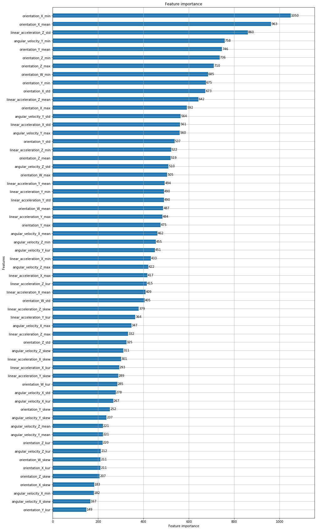
# Removing features with a importance score bellow 400
# The 400 values was chosen from several tests
features_to_remove = []
feat_imp_threshold = 400

# A list of features and importance scores
feat_imp = []
for i in range(len(X_train.columns)):
    feat_imp.append((X_train.columns[i], model_lgb.feature_importances_[i]))

for fi in feat_imp:
    if fi[1] < feat_imp_threshold:
        features_to_remove.append(fi[0])

print(f"Number of feature to be remove: {len(features_to_remove)}\n")
print(features_to_remove)

Number of feature to be remove: 25

['orientation_X_kur', 'orientation_X_skew', 'orientation_Y_kur', 'orientation_Y_skew', 'orientation_Z_std', 'orientation_Z_kur', 'orientation_Z_skew', 'orientation_W_kur', 'orientation_W_skew', 'angular_velocity_X_std', 'angular_velocity_X_min', 'angular_velocity_X_max', 'angular_velocity_X_kur', 'angular_velocity_X_skew', 'angular_velocity_Y_mean', 'angular_velocity_Y_skew', 'angular_velocity_Z_mean', 'angular_velocity_Z_kur', 'angular_velocity_Z_skew', 'linear_acceleration_X_kur', 'linear_acceleration_X_skew', 'linear_acceleration_Y_kur', 'linear_acceleration_Y_skew', 'linear_acceleration_Z_max', 'linear_acceleration_Z_skew']

# Removing features
X_train_v2 = X_train.copy()
X_test_v2 = X_test.copy()

for f in features_to_remove:
    del X_train_v2[f]
    del X_test_v2[f]

X_train_v2.shape, X_test_v2.shape

((3810, 35), (3816, 35))

# Train a new set of models
measured_lgb, predicted_lgb, accuracy_lgb, lgbm_model = train_lgbm_model(X_train_v2, Y_train_encoded, X_test_v2)
print(f"\nMean accuracy for LGBM: {accuracy_lgb}")

Fold: 1 - LGBM Score: 0.8617672790901137
Fold: 2 - LGBM Score: 0.8565179352580927
Fold: 3 - LGBM Score: 0.8442694663167104
Fold: 4 - LGBM Score: 0.8766404199475065
Fold: 5 - LGBM Score: 0.8836395450568679

Mean accuracy for LGBM: 0.8645669291338584

Using the new set of features the mean score was improved by just 1.1%.

Using Random Forest Classifier (RFC)

A random forest is a meta estimator that fits a number of decision tree classifiers on various sub-samples of the dataset and uses averaging to improve the predictive accuracy and control over-fitting.

Documentation: https://scikit-learn.org/stable/modules/generated/sklearn.ensemble.RandomForestClassifier.html

# Function to perform all training steps
def train_rfc(X_train, Y_train, X_test):

    # Create a dictionary that saves the model create in each fold
    models = {}

    # Variables that save the probabilities of each class
    predicted = np.zeros((X_test.shape[0],9))
    measured = np.zeros((X_train.shape[0],9))

    # Use Stratified ShuffleSplit cross-validator
    # Provides train/test indices to split data in train/test sets.
    n_folds = 5
    sss = StratifiedShuffleSplit(n_splits=n_folds, test_size=0.30, random_state=10)

    # Control the number of folds in cross-validation (5 folds)
    k=1

    # Used to compute model accuracy
    all_scores = 0

    # From the generator object gets index for series to use in train and validation
    for train_index, valid_index in sss.split(X_train, Y_train):

        # Saves the split train/validation combinations for each Cross-Validation fold
        X_train_cv, X_validation_cv = X_train.loc[train_index,:], X_train.loc[valid_index,:]
        Y_train_cv, Y_validation_cv = Y_train[train_index], Y_train[valid_index]

        # Training the model
        rfc = RandomForestClassifier(n_estimators=500, min_samples_leaf = 1, max_depth= None, n_jobs=-1, random_state=30)
        rfc.fit(X_train_cv,Y_train_cv)

        # Get the class probabilities of the input samples
        # Save the probabilities for submission
        y_pred = rfc.predict_proba(X_test)
        predicted += y_pred

        # Save the probabilities of validation
        measured[valid_index] = rfc.predict_proba(X_validation_cv)

        # Cumulative sum of the score
        score = rfc.score(X_validation_cv,Y_validation_cv)
        all_scores += score

        print("Fold: {} - RF Score: {}".format(k, score))

        # Saving the model
        models[k] = rfc
        k += 1

    # Compute the mean probability
    predicted /= n_folds
    # Save the mean score value
    mean_score = all_scores/n_folds
    # Save the first trained model
    trained_model = models[1]


    return measured, predicted, mean_score, trained_model

measured_rf, predicted_rf, accuracy_rf, model_rf = train_rfc(X_train_v2, Y_train, X_test_v2)
print(f"\nMean accuracy for RF: {accuracy_rf}")

Fold: 1 - RF Score: 0.863517060367454
Fold: 2 - RF Score: 0.8757655293088364
Fold: 3 - RF Score: 0.8556430446194225
Fold: 4 - RF Score: 0.8775153105861767
Fold: 5 - RF Score: 0.889763779527559

Mean accuracy for RF: 0.8724409448818896

Using Extra-Trees Classifier

The main difference between random forests and extra trees (usually called extreme random forests) lies in the fact that, instead of computing the locally optimal feature/split combination (for the random forest), for each feature under consideration, a random value is selected for the split (for the extra trees).

This leads to more diversified trees and fewer splitters to evaluate when training an extremely random forest.

Documentation: https://scikit-learn.org/stable/modules/generated/sklearn.ensemble.ExtraTreesClassifier.html

# Function to perform all training steps
def train_etc(X_train, Y_train, X_test):

    # Create a dictionary that saves the model create in each fold
    models = {}

    # Variables that save the probabilities of each class
    predicted = np.zeros((X_test.shape[0],9))
    measured = np.zeros((X_train.shape[0],9))

    # Use Stratified ShuffleSplit cross-validator
    # Provides train/test indices to split data in train/test sets.
    n_folds = 5
    sss = StratifiedShuffleSplit(n_splits=n_folds, test_size=0.30, random_state=10)

    # Control the number of folds in cross-validation (5 folds)
    k=1
    all_scores = 0

    # From the generator object gets index for series to use in train and validation
    for train_index, valid_index in sss.split(X_train, Y_train):

        # Saves the split train/validation combinations for each Cross-Validation fold
        X_train_cv, X_validation_cv = X_train.loc[train_index,:], X_train.loc[valid_index,:]
        Y_train_cv, Y_validation_cv = Y_train[train_index], Y_train[valid_index]

        # Training the model
        etc = ExtraTreesClassifier(n_estimators=400, max_depth=10, min_samples_leaf=2, n_jobs=-1, random_state=30)
        etc.fit(X_train_cv,Y_train_cv)

        # Get the class probabilities of the input samples
        # Save the probabilities for submission
        y_pred = etc.predict_proba(X_test)
        predicted += y_pred

        # Save the probabilities of validation
        measured[valid_index] = etc.predict_proba(X_validation_cv)

        # Cumulative sum of the score
        score = etc.score(X_validation_cv,Y_validation_cv)
        all_scores += score

        print("Fold: {} - ET Score: {}".format(k, score))

        # Saving the model
        models[k] = etc
        k += 1

    # Compute the mean probability
    predicted /= n_folds
    # Save the mean score value
    mean_score = all_scores/n_folds
    # Save the first trained model
    trained_model = models[1]


    return measured, predicted, mean_score, trained_model

measured_et, predicted_et, accuracy_et, model_et = train_rfc(X_train_v2, Y_train, X_test_v2)
print(f"\nMean accuracy for ET: {accuracy_et}")

Fold: 1 - RF Score: 0.863517060367454
Fold: 2 - RF Score: 0.8757655293088364
Fold: 3 - RF Score: 0.8556430446194225
Fold: 4 - RF Score: 0.8775153105861767
Fold: 5 - RF Score: 0.889763779527559

Mean accuracy for ET: 0.8724409448818896

Overall results

print(f"LGBM accuracy: {accuracy_lgb}")
print(f"RF accuracy: {accuracy_rf}")
print(f"ET accuracy: {accuracy_et}")

LGBM accuracy: 0.8645669291338584
RF accuracy: 0.8724409448818896
ET accuracy: 0.8724409448818896

For all algorithms used, the mean accuracy was the same.

Let's combine them together to build a new powerful model.

Stacking

Stacking is an ensemble learning technique that combines multiple classifications or regression models via a meta-classifier or a meta-regressor. The base-level models are trained based on a complete training set, then the meta-model is trained on the outputs of the base-level model-like features.

The idea of stacking is to learn several different weak learners (heterogeneous learners) and combine them by training a meta-model to output predictions based on the multiple predictions returned by these weak models.

So, we need to define two things in order to build our stacking model: the L learners we want to fit and the meta-model that combines them.

In our case, the L learns are: LightGBM, Random Forest, and Extra Trees. The meta classifier will be a Logistic Regression model.

# Creatin train and test datasets
x_train = np.concatenate((measured_et, measured_rf, measured_lgb), axis=1)
x_test = np.concatenate((predicted_et, predicted_rf, predicted_lgb), axis=1)

print(x_train.shape, x_test.shape)

(3810, 27) (3816, 27)

# Training the model
from sklearn.linear_model import LogisticRegression
stacker = LogisticRegression(solver="lbfgs", multi_class="auto")
stacker.fit(x_train,Y_train)

# Perform predictions
stacker_pred = stacker.predict_proba(x_test)

# Creating submission file
submission['surface'] =  le.inverse_transform(stacker_pred.argmax(1))
submission.to_csv('submission_stack.csv', index=False)
submission.head()

	series_id	surface
0	0	hard_tiles_large_space
1	1	carpet
2	2	tiled
3	3	soft_tiles
4	4	soft_tiles

References

https://www.researchgate.net/publication/332799607_Surface_Type_Classification_for_Autonomous_Robot_Indoor_Navigation
https://www.kaggle.com/c/career-con-2019/overview
http://mariofilho.com/tutorial-aumentando-o-poder-preditivo-de-seus-modelos-de-machine-learning-com-stacking-ensembles/
https://blog.statsbot.co/ensemble-learning-d1dcd548e936

Classifying the floor surface to help a robot

Comments

My blog

Kaggle: Predict the occurrence of diabetes

More from this blog

The "Vibe Coding" Revolution: Redefining Software Development in 2025

Automated Tests: The Secret to Peaceful Nights

Harness the Power of AI: How ChatGPT Can Boost Your Business Efficiency

MLOps: What it is and why does it Matter?

Basket Icon Detector

Source code

How to use

Classifying the type of flooring surface

Exploratory Data Analysis

Loading the data

Frequency Distribution

Frequency distribution for each column

Feature Engineering

Modeling

Using Gradient Boosting (LightGBM)

Using Random Forest Classifier (RFC)

Using Extra-Trees Classifier

Overall results

Stacking

References

Command Palette

Comments

My blog

Kaggle: Predict the occurrence of diabetes

More from this blog

Source code

How to use

Classifying the type of flooring surface

Exploratory Data Analysis

Loading the data

Frequency Distribution

Frequency distribution for each column

Feature Engineering

Modeling

Using Gradient Boosting (LightGBM)

Using Random Forest Classifier (RFC)

Using Extra-Trees Classifier

Overall results

Stacking

References