This project presents a code/kernel used in a Kaggle competition promoted by Data Science Academy in December of 2019.

The aim of this competition is to build a predictive model that can predict the probability that a particular claim will be approved immediately or not by the insurance company based on the resources available at the beginning of the process, helping the insurance company to accelerate the payment release process and thus provide better service to the client.

Competition page: https://www.kaggle.com/c/competicao-dsa-machine-learning-dec-2019

Building the prediction model

This project aims to build a predictive model that can predict the probability that a particular claim will be approved immediately or not by the insurance company.

The evaluation metric is the log loss.

See the competitions' page for further details.

Below is a detailed description of the developed solution.

Solution

The solution is also available at Github.

You will need Python 3.5+ to run the code.
Python can be downloaded here.
Clone the project locally:

git clone https://github.com/cpatrickalves/kaggle-insurance-claim-classification `

You have to install some Python packages, in command prompt/Terminal:

pip install -r requirements.txt

Access the project folder in command prompt/Terminal and run the following command: jupyter-lab

The datasets are available on the competition's pages.

Files description:

kernel.ipynb - the Jupyter Notebook file with all project workflow (data cleaning, preparation, analysis, machine learning, etc.).
dataset_treino.csv - contains the training dataset with 114,321 rows (claims) and 133 columns (features).
dataset_teste.csv - contains the test dataset with 114,393 rows and 132 columns.
sample_submission.csv - a sample of the submission file.

Loading the datasets

# Loading useful Python packages for Data cleaning and Pre-processing
import numpy as np
import pandas as pd
import pandas_profiling
import matplotlib.pyplot as plt
import category_encoders as ce
from sklearn.preprocessing import MinMaxScaler
from sklearn.preprocessing import RobustScaler
from sklearn.preprocessing import StandardScaler
import seaborn as sns
import warnings
warnings.simplefilter(action='ignore')
pd.set_option('display.max_columns', 150)

# loading datasets
train_df = pd.read_csv('data/dataset_treino.csv')
test_df = pd.read_csv('data/dataset_teste.csv')

train_df.head()

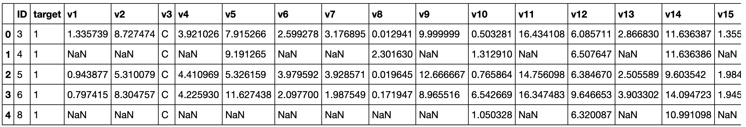
In the following lines, we'll perform several modifications in the datasets, to evaluate the impact of such modifications we'll save each version of the datasets as an object in a dictionary.

data = {}
data['original'] = {'train': train_df, 'test': test_df}

Data Cleaning

The first step before performing any kind of statistical analysis and modeling is to clean the data.

Let's see the type of data we have.

train_df.info()

<class 'pandas.core.frame.DataFrame'>
RangeIndex: 114321 entries, 0 to 114320
Columns: 133 entries, ID to v131
dtypes: float64(108), int64(6), object(19)
memory usage: 116.0+ MB

From the above, we can see that this data set has 114321 rows and 133 columns.

Also, we have 114 numerical features (columns) and 19 categorical features.

Let's see if we have null values (also know as NaN)

# There are null values?
train_df.isnull().values.any()

True

# Null values amount for each column
train_df.isnull().sum().sort_values(ascending=False)

v30       60110
v113      55304
v102      51316
v85       50682
v119      50680
v51       50678
v123      50678
v23       50675
v78       49895
v115      49895
v69       49895
v131      49895
v16       49895
v122      49851
v80       49851
v9        49851
v37       49843
v118      49843
v130      49843
v19       49843
v92       49843
v95       49843
v97       49843
v20       49840
v65       49840
v121      49840
v11       49836
v39       49836
v73       49836
v90       49836
          ...  
v3         3457
v31        3457
v21         611
v22         500
v112        382
v34         111
v40         111
v12          86
v50          86
v10          84
v125         77
v114         30
v14           4
v52           3
v91           3
v107          3
v24           0
v38           0
v47           0
v62           0
v66           0
v129          0
v71           0
v72           0
v74           0
v75           0
v79           0
v110          0
target        0
ID            0
Length: 133, dtype: int64

So, we have a lot of null values in several columns.

Let's check the percentage of null values for each column.

null_values = train_df.isnull().sum()
null_values = round((null_values/train_df.shape[0] * 100), 2)
null_values.sort_values(ascending=False)

v30       52.58
v113      48.38
v102      44.89
v51       44.33
v85       44.33
v23       44.33
v123      44.33
v119      44.33
v115      43.64
v78       43.64
v69       43.64
v131      43.64
v16       43.64
v122      43.61
v80       43.61
v9        43.61
v37       43.60
v130      43.60
v20       43.60
v19       43.60
v92       43.60
v95       43.60
v97       43.60
v65       43.60
v118      43.60
v121      43.60
v53       43.59
v42       43.59
v68       43.59
v67       43.59
          ...  
v3         3.02
v31        3.02
v21        0.53
v22        0.44
v112       0.33
v40        0.10
v34        0.10
v12        0.08
v50        0.08
v125       0.07
v10        0.07
v114       0.03
v129       0.00
target     0.00
v107       0.00
v14        0.00
v24        0.00
v38        0.00
v47        0.00
v52        0.00
v62        0.00
v66        0.00
v71        0.00
v72        0.00
v74        0.00
v75        0.00
v79        0.00
v91        0.00
v110       0.00
ID         0.00
Length: 133, dtype: float64

Considering that we are dealing with anonymous data and we can't know the meaning of the data, I'll remove all columns with more than 40% of null values.

# Get the names of the columns that have more than 40% of null values
high_nan_rate_columns = null_values[null_values > 40].index

# Make a copy if the original datasets and remove the columns
train_df_cleaned = train_df.copy()
test_df_cleaned = test_df.copy()
train_df_cleaned.drop(high_nan_rate_columns, axis=1, inplace=True)
test_df_cleaned.drop(high_nan_rate_columns, axis=1, inplace=True)

# Remove the ID column (it is not useful for modeling)
train_df_cleaned.drop(['ID'], axis=1, inplace=True)

train_df_cleaned.info()

<class 'pandas.core.frame.DataFrame'>
RangeIndex: 114321 entries, 0 to 114320
Data columns (total 30 columns):
target    114321 non-null int64
v3        110864 non-null object
v10       114237 non-null float64
v12       114235 non-null float64
v14       114317 non-null float64
v21       113710 non-null float64
v22       113821 non-null object
v24       114321 non-null object
v31       110864 non-null object
v34       114210 non-null float64
v38       114321 non-null int64
v40       114210 non-null float64
v47       114321 non-null object
v50       114235 non-null float64
v52       114318 non-null object
v56       107439 non-null object
v62       114321 non-null int64
v66       114321 non-null object
v71       114321 non-null object
v72       114321 non-null int64
v74       114321 non-null object
v75       114321 non-null object
v79       114321 non-null object
v91       114318 non-null object
v107      114318 non-null object
v110      114321 non-null object
v112      113939 non-null object
v114      114291 non-null float64
v125      114244 non-null object
v129      114321 non-null int64
dtypes: float64(8), int64(5), object(17)
memory usage: 26.2+ MB

Now we have only 30 columns in the data set.

But we still have null values that need to be handled.

null_values_columns = train_df_cleaned.isnull().sum().sort_values(ascending=False)
null_values_columns = null_values_columns[null_values_columns > 0]
null_values_columns

v56     6882
v31     3457
v3      3457
v21      611
v22      500
v112     382
v40      111
v34      111
v50       86
v12       86
v10       84
v125      77
v114      30
v14        4
v91        3
v107       3
v52        3
dtype: int64

train_df_cleaned[null_values_columns.index].info()

<class 'pandas.core.frame.DataFrame'>
RangeIndex: 114321 entries, 0 to 114320
Data columns (total 17 columns):
v56     107439 non-null object
v31     110864 non-null object
v3      110864 non-null object
v21     113710 non-null float64
v22     113821 non-null object
v112    113939 non-null object
v40     114210 non-null float64
v34     114210 non-null float64
v50     114235 non-null float64
v12     114235 non-null float64
v10     114237 non-null float64
v125    114244 non-null object
v114    114291 non-null float64
v14     114317 non-null float64
v91     114318 non-null object
v107    114318 non-null object
v52     114318 non-null object
dtypes: float64(8), object(9)
memory usage: 14.8+ MB

From the above, there are 8 numeric columns and 9 categorical columns with null values.

For now, we will replace the null values by the MEAN value for each numeric column and for the MODE for each of the categorical columns.

###### TRAIN DATASET ######

##### Numerical columns
null_values_columns_train = train_df_cleaned.isnull().sum().sort_values(ascending=False)
numerical_col_null_values = train_df_cleaned[null_values_columns_train.index].select_dtypes(include=['float64', 'int64']).columns
# for each column
for c in numerical_col_null_values:
    # Get the mean
    mean = train_df_cleaned[c].mean()
    # replace the NaN by mode
    train_df_cleaned[c].fillna(mean, inplace=True)

##### Categorical columns
categ_col_null_values = train_df_cleaned[null_values_columns_train.index].select_dtypes(include=['object']).columns
# for each column
for c in categ_col_null_values:
    # Get the most frequent value (mode)
    mode = train_df_cleaned[c].value_counts().index[0]
    # replace the NaN by mode
    train_df_cleaned[c].fillna(mode, inplace=True)


###### TEST DATASET ######

##### Numerical columns
null_values_columns_test = test_df_cleaned.isnull().sum().sort_values(ascending=False)
#print(null_values_columns_test)
numerical_col_null_values = list(test_df_cleaned[null_values_columns_test.index].select_dtypes(include=['float64', 'int64']).columns)
numerical_col_null_values.remove('ID')
# for each column
for c in numerical_col_null_values:
    # Get the mean
    mean = test_df_cleaned[c].mean()
    # replace the NaN by mode
    test_df_cleaned[c].fillna(mean, inplace=True)

##### Categorical columns
categ_col_null_values = test_df_cleaned[null_values_columns_test.index].select_dtypes(include=['object']).columns
# for each column
for c in categ_col_null_values:
    # Get the most frequent value (mode)
    mode = test_df_cleaned[c].value_counts().index[0]
    # replace the NaN by mode
    test_df_cleaned[c].fillna(mode, inplace=True)

# There are null values?
print(train_df_cleaned.isnull().values.any())
print(test_df_cleaned.isnull().values.any())

False
False

# Save the list of current columns
selected_columns = list(train_df_cleaned.columns)
selected_columns_test = selected_columns[:]
selected_columns_test.remove('target')
selected_columns_test.append('ID')

# Filter the columns in the test dataset
test_df_cleaned = test_df_cleaned[list(selected_columns_test)]

# Save the datasets in dict
data['cleaned_v1'] = {'train': train_df_cleaned.copy(), 'test':test_df_cleaned.copy()}

Data Analysis

Now that the dataset is cleaned, let's compute some statistics about the data and perform the transformations.

We'll use the Pandas Profiling library to create a report about the data.

%%time
train_df_cleaned.profile_report(style={'full_width':True})

This procedure generates a 17 MB file with the report, to see it, download the HTML version of the kernel here.

From the report, we can see some issues in the dataset.

There are features highly correlated, with a lot of zero values and with high cardinality.

Let's check each one of these issues and see if we should remove or transform these features.

Features highly correlated

From report the following features are highly correlated:

v12 is highly correlated with v10 (ρ = 0.9117725571)
v34 is highly correlated with v114 (ρ = 0.9118410589)

These high correlations could mean that the features are multicollinear.

Multicollinearity happens when one predictor variable in a multiple regression model can be linearly predicted from the others with a high degree of accuracy. This can lead to model overfitting and skewed or misleading results.

So, we need to remove some of these features. As we don't know the meaning of the features, for now, we will just remove the v12 and v114. We can come back to this latter and change the removed features to see the impact in results.

selected_columns = list(train_df_cleaned.columns)
# Remove the selected columns
selected_columns.remove('v12')
selected_columns.remove('v114')

Features with highly cardinality

From the report, the following categorical features have high cardinality:

v125 has a high cardinality: 90 distinct values
v22 has a high cardinality: 18210 distinct values
v56 has a high cardinality: 122 distinct values
v112 has a high cardinality: 22 distinct values

High cardinality means that the categorical feature has a large number of distinct values.

Features with high cardinality are hard to encode.

For now, we'll remove them.

# Remove the selected columns
selected_columns.remove('v125')
selected_columns.remove('v22')
selected_columns.remove('v112')
selected_columns.remove('v56')

# Save the list of current columns
selected_columns_test = selected_columns[:]
selected_columns_test.remove('target')
selected_columns_test.append('ID')

# Filter the columns in the train dataset
train_df_cleaned = train_df_cleaned[selected_columns].copy()
# Filter the columns in the test dataset
test_df_cleaned = test_df_cleaned[selected_columns_test].copy()

# Save the datasets in dict
data['cleaned_v2'] = {'train': train_df_cleaned.copy(), 'test':test_df_cleaned.copy()}

Features with many zeros.

From the report, the following numerical features have high number of zeros:

v129 has 90247 (78.9%) zeros
v38 has 109724 (96.0%) zeros
v62 has 20630 (18.0%) zeros
v72 has 3355 (2.9%) zeros

Again, we don't know the meaning of these features, we can't tell what the high number of zeros could mean.

As the features v129 and v38 are zero for almost all rows, we'll remove them.

# Remove the selected columns
selected_columns.remove('v129')
selected_columns.remove('v38')
selected_columns

['target',
 'v3',
 'v10',
 'v14',
 'v21',
 'v24',
 'v31',
 'v34',
 'v40',
 'v47',
 'v50',
 'v52',
 'v62',
 'v66',
 'v71',
 'v72',
 'v74',
 'v75',
 'v79',
 'v91',
 'v107',
 'v110']

# Save the list of current columns
selected_columns_test = selected_columns[:]
selected_columns_test.remove('target')
selected_columns_test.append('ID')

# Filter the columns in the train dataset
train_df_cleaned = train_df_cleaned[selected_columns].copy()
# Filter the columns in the test dataset
test_df_cleaned = test_df_cleaned[selected_columns_test].copy()

# Save the datasets in dict
data['cleaned_v3'] = {'train': train_df_cleaned.copy(), 'test': test_df_cleaned.copy()}

Feature Engineering

Now, it's time to transform our data to feed some machine learning models.

Enconding categorical features

Some ML algorithms can't handle categorical features (ex: Logistic Regression, SVM, etc.)

Better encoding of categorical data can mean better model performance.

There are different methods for encoding nominal and ordinal data. But as we don't know the meaning of categorical features we'll consider all categorical features as nominal.

For nominal columns, we can use methods like OneHot, Hashing, LeaveOneOut, and Target encoding. But we should avoid OneHot for high cardinality columns and decision tree-based algorithms.

First, let's compute the cardinality for categorical features.

train_df_cleaned = data['cleaned_v2']['train'].copy()
test_df_cleaned = data['cleaned_v2']['test'].copy()
train_df_cleaned.select_dtypes(include=['object']).columns

Index(['v3', 'v24', 'v31', 'v47', 'v52', 'v66', 'v71', 'v74', 'v75', 'v79',
       'v91', 'v107', 'v110'],
      dtype='object')

# Before encoding categorical variables we need to convert the categorical data from "object" to "category"
# Train
for col_name in train_df_cleaned.select_dtypes(include=['object']).columns:    
    train_df_cleaned[col_name] = train_df_cleaned[col_name].astype('category')

# Test
for col_name in test_df_cleaned.select_dtypes(include=['object']).columns:
    test_df_cleaned[col_name] = test_df_cleaned[col_name].astype('category')

train_df_cleaned.select_dtypes(include=['category']).describe()

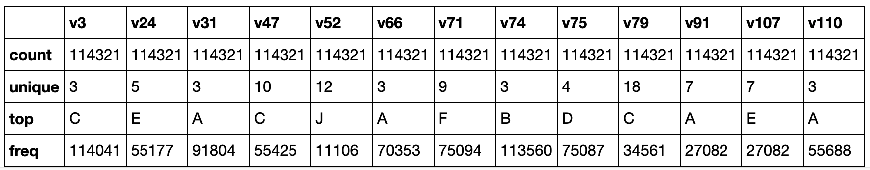
One of the most used encoding methods for nominal data is the OneHot, where each unique value is converted into a new column with 1 or a 0 denoting the presence or absence of this value. But, this method creates a new column for each unique value in the column, so if the cardinality is high, the number of new columns could lead us to new issues due to the number of features.

Columns v47, v52, v71, v91, v107, and v79 have high cardinality, so they need special treatment.

In the following lines, we'll split the datasets into three versions, one with the OneHot applied in all categorical columns, another version with OneHot applied to the low cardinality features, and Hashing to the high cardinality variables, and the last where all categorical variables are removed.

##### VERSION 1
# Encoding all categorical variables with OneHot
cat_columns = ['v3', 'v24',  'v31', 'v66', 'v74', 'v75', 'v110', 'v47', 'v52','v71', 'v91', 'v107', 'v79']
ce_onehot = ce.OneHotEncoder(cols=cat_columns)

# For columns v47 and v79, the are some values only present in the train dataset. Thus, the enconding process create a different number of columns 
# in train and test dataset and prevents the model prediction. So before save the datasets I remove the extra columns 'v47_10', 'v79_18'.
# Apply the encoding
data['cleaned_transformed_CatgEncoded_v1'] = {'train':ce_onehot.fit_transform(train_df_cleaned).drop(['v47_10', 'v79_18'], axis=1), 
                                              'test': ce_onehot.fit_transform(test_df_cleaned)}

print(data['cleaned_transformed_CatgEncoded_v1']['train'].columns)
print(data['cleaned_transformed_CatgEncoded_v1']['test'].columns)

Index(['target', 'v3_1', 'v3_2', 'v3_3', 'v10', 'v14', 'v21', 'v24_1', 'v24_2',
       'v24_3', 'v24_4', 'v24_5', 'v31_1', 'v31_2', 'v31_3', 'v34', 'v38',
       'v40', 'v47_1', 'v47_2', 'v47_3', 'v47_4', 'v47_5', 'v47_6', 'v47_7',
       'v47_8', 'v47_9', 'v50', 'v52_1', 'v52_2', 'v52_3', 'v52_4', 'v52_5',
       'v52_6', 'v52_7', 'v52_8', 'v52_9', 'v52_10', 'v52_11', 'v52_12', 'v62',
       'v66_1', 'v66_2', 'v66_3', 'v71_1', 'v71_2', 'v71_3', 'v71_4', 'v71_5',
       'v71_6', 'v71_7', 'v71_8', 'v71_9', 'v72', 'v74_1', 'v74_2', 'v74_3',
       'v75_1', 'v75_2', 'v75_3', 'v75_4', 'v79_1', 'v79_2', 'v79_3', 'v79_4',
       'v79_5', 'v79_6', 'v79_7', 'v79_8', 'v79_9', 'v79_10', 'v79_11',
       'v79_12', 'v79_13', 'v79_14', 'v79_15', 'v79_16', 'v79_17', 'v91_1',
       'v91_2', 'v91_3', 'v91_4', 'v91_5', 'v91_6', 'v91_7', 'v107_1',
       'v107_2', 'v107_3', 'v107_4', 'v107_5', 'v107_6', 'v107_7', 'v110_1',
       'v110_2', 'v110_3', 'v129'],
      dtype='object')
Index(['v3_1', 'v3_2', 'v3_3', 'v10', 'v14', 'v21', 'v24_1', 'v24_2', 'v24_3',
       'v24_4', 'v24_5', 'v31_1', 'v31_2', 'v31_3', 'v34', 'v38', 'v40',
       'v47_1', 'v47_2', 'v47_3', 'v47_4', 'v47_5', 'v47_6', 'v47_7', 'v47_8',
       'v47_9', 'v50', 'v52_1', 'v52_2', 'v52_3', 'v52_4', 'v52_5', 'v52_6',
       'v52_7', 'v52_8', 'v52_9', 'v52_10', 'v52_11', 'v52_12', 'v62', 'v66_1',
       'v66_2', 'v66_3', 'v71_1', 'v71_2', 'v71_3', 'v71_4', 'v71_5', 'v71_6',
       'v71_7', 'v71_8', 'v71_9', 'v72', 'v74_1', 'v74_2', 'v74_3', 'v75_1',
       'v75_2', 'v75_3', 'v75_4', 'v79_1', 'v79_2', 'v79_3', 'v79_4', 'v79_5',
       'v79_6', 'v79_7', 'v79_8', 'v79_9', 'v79_10', 'v79_11', 'v79_12',
       'v79_13', 'v79_14', 'v79_15', 'v79_16', 'v79_17', 'v91_1', 'v91_2',
       'v91_3', 'v91_4', 'v91_5', 'v91_6', 'v91_7', 'v107_1', 'v107_2',
       'v107_3', 'v107_4', 'v107_5', 'v107_6', 'v107_7', 'v110_1', 'v110_2',
       'v110_3', 'v129', 'ID'],
      dtype='object')

##### VERSION 2
# Encoding categorical variables with low cardinality with OneHot
low_cardinality_columns = ['v3', 'v24',  'v31', 'v66', 'v74', 'v75', 'v110']
ce_onehot = ce.OneHotEncoder(cols=low_cardinality_columns)

# Apply the encoding 
train_df_cleaned_transformed = ce_onehot.fit_transform(train_df_cleaned)
test_df_cleaned_transformed = ce_onehot.fit_transform(test_df_cleaned)

For the categorical features with high cardinality, we will use the Hashing method.

# Encoding categorical variables with high cardinality with Hashing
high_cardinality_columns = ['v47', 'v52','v71', 'v91', 'v107', 'v79']

#train_df_cleaned_transformed[high_cardinality_columns].describe().loc['unique']

ce_hash = ce.HashingEncoder(max_process=1, cols = high_cardinality_columns, n_components=12)
train_df_cleaned_transformed = ce_hash.fit_transform(train_df_cleaned_transformed)
test_df_cleaned_transformed = ce_hash.fit_transform(test_df_cleaned_transformed)

data['cleaned_transformed_CatgEncoded_v2'] = {'train': train_df_cleaned_transformed.copy(), 'test': test_df_cleaned_transformed.copy()}

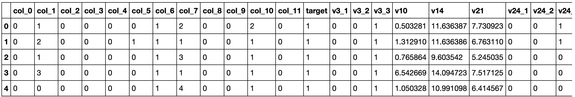
train_df_cleaned_transformed.head(5)

##### VERSION 3
# Removing all categorical variables with OneHot
cat_columns = ['v3', 'v24',  'v31', 'v66', 'v74', 'v75', 'v110', 'v47', 'v52','v71', 'v91', 'v107', 'v79']

# Apply the encoding
data['cleaned_dropCatg'] = {'train':train_df_cleaned.drop(columns=cat_columns, axis=1), 
                               'test': test_df_cleaned.drop(columns=cat_columns, axis=1)}

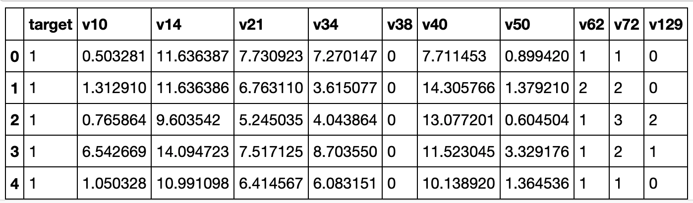
data['cleaned_dropCatg']['train'].head()

Transforming numerical features

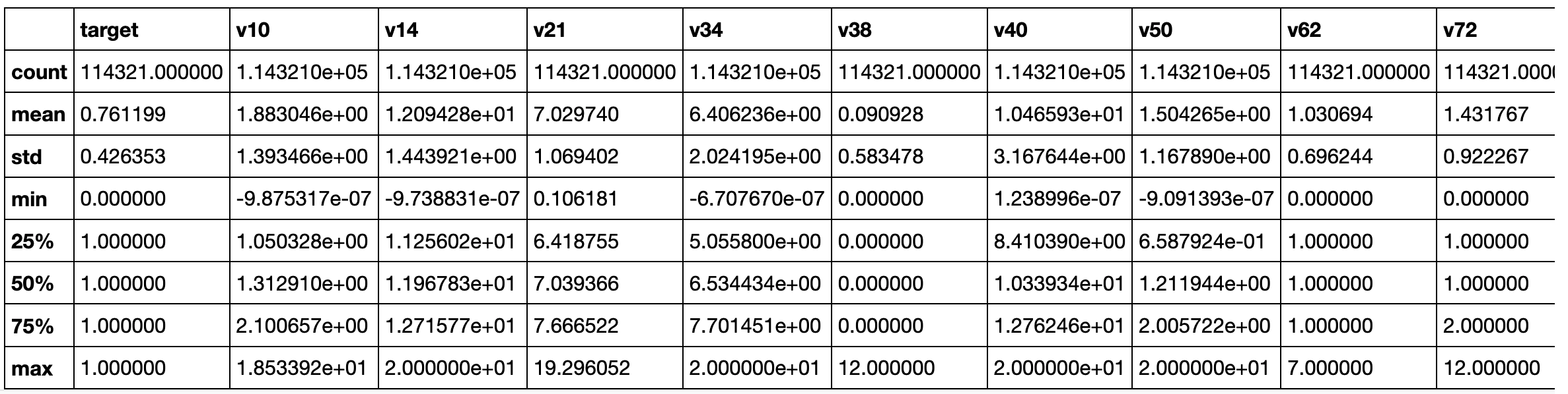
Let's check the numerical features.

train_df_cleaned.select_dtypes(exclude=['category']).describe()

# Plot the distribution of numerical features

# Create fig object
fig, axes = plt.subplots(2, 5, figsize=(20,8))

numerical_columns = train_df_cleaned.select_dtypes(exclude=['category']).columns
numerical_columns = list(numerical_columns)
numerical_columns.remove('target')

# Create a plot for each feature
x,y = 0,0
for i, column in enumerate(numerical_columns):

    sns.distplot(train_df_cleaned[column], ax=axes[x,y])
    if i < 4:
        y += 1
    elif i==4:
        x = 1
        y = 0
    else:
        y+=1

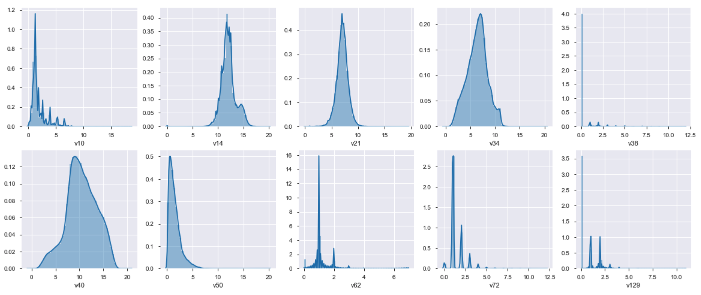
There are several transformations to be applied in these features, as the datasets are not that bigger, we'll apply MinMaxScaler(), RobustScaler(), StandardScaler().

MinMaxScaler subtracts the minimum value in the column and then divides by the difference between the original maximum and original minimum.
RobustScaler standardizes a feature by removing the median and dividing each feature by the interquartile range.
StandardScaler standardizes a feature by removing the mean and dividing each value by the standard deviation.

# Apply all scalings methods
scaling = {'MinMaxScaler': MinMaxScaler(),
         'RobustScaler': RobustScaler(),
         'StandardScaler': StandardScaler()
        }

# Temporarily save transformed data sets
temp_dict = {}

# Save the list of the numerical columns of the original dataset
num_cols = list(data['original']['train'].select_dtypes(exclude=['object']).columns)

# Apply all scalings in all datasets
for d in data.keys():
    print(f"Scaling dataset: {d}")

    # Get the list of numerical columns
    cols_train = list(data[d]['train'].select_dtypes(exclude=['category','object']).columns)
    cols_test = list(data[d]['test'].select_dtypes(exclude=['category','object']).columns)
    cols_train.remove('target')

    # As the encoding process of categorical features create numerical columns
    # we need to filter these columns    
    cols_train = list(set(num_cols) & set(cols_train))
    cols_test = list(set(num_cols) & set(cols_test))
    cols_test.remove('ID')

    # Apply Transformations
    for s in scaling.keys():
        print(f"   Applying {s}() ...")    

        # Make a copy of the original DFs
        train = data[d]['train'].copy()
        test = data[d]['test'].copy()
        # Apply scaling
        train[cols_train] = scaling[s].fit_transform(train[cols_train])
        test[cols_test] = scaling[s].fit_transform(test[cols_test])    
        # Save the data
        temp_dict[f"{d}_{s}"] = {'train': train.copy(), 'test': test.copy()}

# Save the new datasets in data dict        
data.update(temp_dict)        
print(data.keys())

Scaling dataset: original
   Applying MinMaxScaler() ...
   Applying RobustScaler() ...
   Applying StandardScaler() ...
Scaling dataset: cleaned_v1
   Applying MinMaxScaler() ...
   Applying RobustScaler() ...
   Applying StandardScaler() ...
Scaling dataset: cleaned_v2
   Applying MinMaxScaler() ...
   Applying RobustScaler() ...
   Applying StandardScaler() ...
Scaling dataset: cleaned_v3
   Applying MinMaxScaler() ...
   Applying RobustScaler() ...
   Applying StandardScaler() ...
Scaling dataset: cleaned_transformed_CatgEncoded_v1
   Applying MinMaxScaler() ...
   Applying RobustScaler() ...
   Applying StandardScaler() ...
Scaling dataset: cleaned_transformed_CatgEncoded_v2
   Applying MinMaxScaler() ...
   Applying RobustScaler() ...
   Applying StandardScaler() ...
Scaling dataset: cleaned_dropCatg
   Applying MinMaxScaler() ...
   Applying RobustScaler() ...
   Applying StandardScaler() ...
dict_keys(['original', 'cleaned_v1', 'cleaned_v2', 'cleaned_v3', 'cleaned_transformed_CatgEncoded_v1', 'cleaned_transformed_CatgEncoded_v2', 'cleaned_dropCatg', 'original_MinMaxScaler', 'original_RobustScaler', 'original_StandardScaler', 'cleaned_v1_MinMaxScaler', 'cleaned_v1_RobustScaler', 'cleaned_v1_StandardScaler', 'cleaned_v2_MinMaxScaler', 'cleaned_v2_RobustScaler', 'cleaned_v2_StandardScaler', 'cleaned_v3_MinMaxScaler', 'cleaned_v3_RobustScaler', 'cleaned_v3_StandardScaler', 'cleaned_transformed_CatgEncoded_v1_MinMaxScaler', 'cleaned_transformed_CatgEncoded_v1_RobustScaler', 'cleaned_transformed_CatgEncoded_v1_StandardScaler', 'cleaned_transformed_CatgEncoded_v2_MinMaxScaler', 'cleaned_transformed_CatgEncoded_v2_RobustScaler', 'cleaned_transformed_CatgEncoded_v2_StandardScaler', 'cleaned_dropCatg_MinMaxScaler', 'cleaned_dropCatg_RobustScaler', 'cleaned_dropCatg_StandardScaler'])

Machine Learning

Now, let's fit the datasets in some machine learning models.

# Importing packages
from sklearn.model_selection import train_test_split, GridSearchCV, KFold
from sklearn.feature_selection import SelectFromModel
from sklearn.metrics import accuracy_score, confusion_matrix, classification_report, roc_auc_score, log_loss
from sklearn.model_selection import StratifiedShuffleSplit
from sklearn.linear_model import LogisticRegression
from sklearn.discriminant_analysis import LinearDiscriminantAnalysis
from sklearn.naive_bayes import GaussianNB
from sklearn.neighbors import KNeighborsClassifier
from sklearn.svm import SVC
from sklearn.ensemble import RandomForestClassifier
from sklearn.ensemble import ExtraTreesClassifier
from sklearn.calibration import CalibratedClassifierCV
from xgboost.sklearn import XGBClassifier
from xgboost import plot_importance
from imblearn.over_sampling import SMOTE, ADASYN
from numpy import sort
import lightgbm as lgb
import xgboost as xgb

len(data)

We have more than 20 datasets to test on the machine learning models.

Not all machine learning algorithms can be used with all datasets, some of them, like SVM, required scaling the numerical data.

So we'll filter the datasets used in training/tests.

# A function to run train and test for each model
def run_model(name, model, X_train, Y_train, cv_folds=5, verbose=True):   

    if verbose: print(f"{name}")

    # Use Stratified ShuffleSplit cross-validator
    # Provides train/test indices to split data in train/test sets.
    n_folds = 5
    sss = StratifiedShuffleSplit(n_splits=cv_folds, test_size=0.30, random_state=10)

    # Control the number of folds in cross-validation (5 folds)
    k=1

    acc = 0
    roc = 0
    log_loss_score = 0

    # From the generator object gets index for series to use in train and validation
    for train_index, valid_index in sss.split(X_train, Y_train):

        # Saves the split train/validation combinations for each Cross-Validation fold
        X_train_cv, X_validation_cv = X_train.loc[train_index,:], X_train.loc[valid_index,:]
        Y_train_cv, Y_validation_cv = Y_train[train_index], Y_train[valid_index]

        #print(f"Fold: {k}") 
        # Training the model
        try:
            model.fit(X_train_cv, Y_train_cv, eval_set=[(X_train_cv, Y_train_cv), (X_validation_cv, Y_validation_cv)], eval_metric='logloss', verbose=False )        
        except:
            try: 
                model.fit(X_train_cv, Y_train_cv, eval_set=[(X_train_cv, Y_train_cv), (X_validation_cv, Y_validation_cv)], verbose=False)        
            except:
                try:
                    model.fit(X_train_cv, Y_train_cv, verbose=False)
                except:
                    model.fit(X_train_cv, Y_train_cv)

        # Get the class probabilities of the input samples        
        train_pred = model.predict(X_validation_cv)
        train_pred_prob = model.predict_proba(X_validation_cv)[:,1]

        acc += accuracy_score(Y_validation_cv, train_pred)
        roc += roc_auc_score(Y_validation_cv, train_pred_prob)
        log_loss_score += log_loss(Y_validation_cv, train_pred_prob)   

        k += 1

    # Compute the mean
    if verbose:
        print("Accuracy : %.4g" % (acc/(k-1)))
        print("AUC Score: %f" % (roc/(k-1)))
        print("Log Loss: %f" % (log_loss_score/(k-1)))
        print("-"*30)

    # Return the last version 
    return (model, log_loss_score/(k-1))

print(list(data.keys()))

['original', 'cleaned_v1', 'cleaned_v2', 'cleaned_v3', 'cleaned_transformed_CatgEncoded_v1', 'cleaned_transformed_CatgEncoded_v2', 'cleaned_dropCatg', 'original_MinMaxScaler', 'original_RobustScaler', 'original_StandardScaler', 'cleaned_v1_MinMaxScaler', 'cleaned_v1_RobustScaler', 'cleaned_v1_StandardScaler', 'cleaned_v2_MinMaxScaler', 'cleaned_v2_RobustScaler', 'cleaned_v2_StandardScaler', 'cleaned_v3_MinMaxScaler', 'cleaned_v3_RobustScaler', 'cleaned_v3_StandardScaler', 'cleaned_transformed_CatgEncoded_v1_MinMaxScaler', 'cleaned_transformed_CatgEncoded_v1_RobustScaler', 'cleaned_transformed_CatgEncoded_v1_StandardScaler', 'cleaned_transformed_CatgEncoded_v2_MinMaxScaler', 'cleaned_transformed_CatgEncoded_v2_RobustScaler', 'cleaned_transformed_CatgEncoded_v2_StandardScaler', 'cleaned_dropCatg_MinMaxScaler', 'cleaned_dropCatg_RobustScaler', 'cleaned_dropCatg_StandardScaler']

We'll choose all datasets with scaled and cleaned data and will try several classification models as described below.

models = {}

# From the previous analysis I see that KNN, Random Forest, and Extra Trees had poor results and SVM took too long to run, I'll remove them from the model's list

models['LogisticRegression'] = LogisticRegression()
models['LinearDiscriminantAnalysis'] = LinearDiscriminantAnalysis()
#models['KNeighborsClassifier'] = KNeighborsClassifier(n_jobs=-1)
#models['SVM'] = SVC(probability=True)
#models['RandomForestClassifier'] = RandomForestClassifier(n_jobs=-1)
#models['ExtraTreesClassifier'] = ExtraTreesClassifier(n_jobs=-1)
models['LGBMClassifier'] = lgb.LGBMClassifier(objective='binary', 
                                              is_unbalance=True, 
                                              max_depth=30, 
                                              learning_rate=0.05, 
                                              n_estimators=500, 
                                              num_leaves=30,
                                             verbose = 0)

# The model parameters were taken from https://www.kaggle.com/rodrigolima82/kernel-xgboost-otimizado
# Thanks Rodrigo Lima for sharing his kernel
models['XGBClassifier'] = XGBClassifier(learning_rate = 0.1,
                          n_estimators = 200,
                          max_depth = 5,
                          min_child_weight = 1,
                          gamma = 0,
                          subsample = 0.8,
                          colsample_bytree = 0.8,
                          objective = 'binary:logistic',
                          n_jobs = -1,
                          scale_pos_weight = 1,
                          verbose = False,
                          seed = 32)


# When performing classification you often want to predict not only the class label, but also the associated probability. 
# This probability gives you some kind of confidence on the prediction. 
# However, not all classifiers provide well-calibrated probabilities, some being over-confident while others being under-confident. 
# Thus, a separate calibration of predicted probabilities is often desirable as a postprocessing.
#models['Calibrated_LogisticRegression'] = CalibratedClassifierCV(LogisticRegression())
#models['Calibrated_LinearDiscriminantAnalysis'] = CalibratedClassifierCV(LinearDiscriminantAnalysis())
#models['Calibrated_KNeighborsClassifier'] = CalibratedClassifierCV(KNeighborsClassifier(n_jobs=-1))
#models['Calibrated_SVM'] = CalibratedClassifierCV(models['SVM'])

# Splitting features and targets for train data
datasets = ['cleaned_transformed_CatgEncoded_v1_MinMaxScaler', 'cleaned_transformed_CatgEncoded_v1_RobustScaler', 
            'cleaned_transformed_CatgEncoded_v1_StandardScaler', 'cleaned_transformed_CatgEncoded_v2_MinMaxScaler', 
            'cleaned_transformed_CatgEncoded_v2_RobustScaler', 'cleaned_transformed_CatgEncoded_v2_StandardScaler', 
            'cleaned_dropCatg_MinMaxScaler', 'cleaned_dropCatg_RobustScaler', 'cleaned_dropCatg_StandardScaler']

results = pd.DataFrame(columns=['Dataset', 'Model', 'Logloss'])

# loop through all datasets and ML models
for d in datasets:
    train = data[d]['train']
    train_x = train.drop(['target'], axis=1)
    train_y = train['target']

    print(f'###### DATASET: {d} ######')

    for m in models.keys():
        # Train and test the model
        models[m], log_loss_result = run_model(m, models[m], train_x, train_y)  

        # Save Results
        results = results.append({'Dataset' : d , 'Model' : m, 'Logloss': log_loss_result} , ignore_index=True)

###### DATASET: cleaned_transformed_CatgEncoded_v1_MinMaxScaler ######
LogisticRegression
Accuracy : 0.7744
AUC Score: 0.729911
Log Loss: 0.487398
------------------------------
LinearDiscriminantAnalysis
Accuracy : 0.7702
AUC Score: 0.723778
Log Loss: 0.490958
------------------------------
LGBMClassifier
Accuracy : 0.6692
AUC Score: 0.748472
Log Loss: 0.573621
------------------------------
XGBClassifier
Accuracy : 0.7816
AUC Score: 0.749879
Log Loss: 0.468973
------------------------------
###### DATASET: cleaned_transformed_CatgEncoded_v1_RobustScaler ######
LogisticRegression
Accuracy : 0.7753
AUC Score: 0.730191
Log Loss: 0.487333
------------------------------
LinearDiscriminantAnalysis
Accuracy : 0.7702
AUC Score: 0.723778
Log Loss: 0.490958
------------------------------
LGBMClassifier
Accuracy : 0.6685
AUC Score: 0.748429
Log Loss: 0.573623
------------------------------
XGBClassifier
Accuracy : 0.7817
AUC Score: 0.749515
Log Loss: 0.469239
------------------------------
###### DATASET: cleaned_transformed_CatgEncoded_v1_StandardScaler ######
LogisticRegression
Accuracy : 0.7752
AUC Score: 0.730168
Log Loss: 0.487344
------------------------------
LinearDiscriminantAnalysis
Accuracy : 0.7702
AUC Score: 0.723778
Log Loss: 0.490958
------------------------------
LGBMClassifier
Accuracy : 0.6692
AUC Score: 0.748610
Log Loss: 0.573528
------------------------------
XGBClassifier
Accuracy : 0.7817
AUC Score: 0.749643
Log Loss: 0.469190
------------------------------
###### DATASET: cleaned_transformed_CatgEncoded_v2_MinMaxScaler ######
LogisticRegression
Accuracy : 0.7742
AUC Score: 0.729582
Log Loss: 0.487827
------------------------------
LinearDiscriminantAnalysis
Accuracy : 0.7693
AUC Score: 0.723832
Log Loss: 0.491422
------------------------------
LGBMClassifier
Accuracy : 0.6692
AUC Score: 0.748208
Log Loss: 0.573921
------------------------------
XGBClassifier
Accuracy : 0.7817
AUC Score: 0.749010
Log Loss: 0.469626
------------------------------
###### DATASET: cleaned_transformed_CatgEncoded_v2_RobustScaler ######
LogisticRegression
Accuracy : 0.7753
AUC Score: 0.729843
Log Loss: 0.487758
------------------------------
LinearDiscriminantAnalysis
Accuracy : 0.7693
AUC Score: 0.723832
Log Loss: 0.491422
------------------------------
LGBMClassifier
Accuracy : 0.6687
AUC Score: 0.748150
Log Loss: 0.573849
------------------------------
XGBClassifier
Accuracy : 0.7813
AUC Score: 0.748885
Log Loss: 0.469714
------------------------------
###### DATASET: cleaned_transformed_CatgEncoded_v2_StandardScaler ######
LogisticRegression
Accuracy : 0.7753
AUC Score: 0.729860
Log Loss: 0.487754
------------------------------
LinearDiscriminantAnalysis
Accuracy : 0.7693
AUC Score: 0.723832
Log Loss: 0.491422
------------------------------
LGBMClassifier
Accuracy : 0.669
AUC Score: 0.748118
Log Loss: 0.573951
------------------------------
XGBClassifier
Accuracy : 0.7814
AUC Score: 0.748688
Log Loss: 0.469767
------------------------------
###### DATASET: cleaned_dropCatg_MinMaxScaler ######
LogisticRegression
Accuracy : 0.7613
AUC Score: 0.704112
Log Loss: 0.503248
------------------------------
LinearDiscriminantAnalysis
Accuracy : 0.7612
AUC Score: 0.700375
Log Loss: 0.506688
------------------------------
LGBMClassifier
Accuracy : 0.6533
AUC Score: 0.719685
Log Loss: 0.601128
------------------------------
XGBClassifier
Accuracy : 0.7745
AUC Score: 0.721859
Log Loss: 0.489468
------------------------------
###### DATASET: cleaned_dropCatg_RobustScaler ######
LogisticRegression
Accuracy : 0.7615
AUC Score: 0.704325
Log Loss: 0.503206
------------------------------
LinearDiscriminantAnalysis
Accuracy : 0.7612
AUC Score: 0.700375
Log Loss: 0.506688
------------------------------
LGBMClassifier
Accuracy : 0.6531
AUC Score: 0.720171
Log Loss: 0.600992
------------------------------
XGBClassifier
Accuracy : 0.7743
AUC Score: 0.721641
Log Loss: 0.489606
------------------------------
###### DATASET: cleaned_dropCatg_StandardScaler ######
LogisticRegression
Accuracy : 0.7615
AUC Score: 0.704326
Log Loss: 0.503205
------------------------------
LinearDiscriminantAnalysis
Accuracy : 0.7612
AUC Score: 0.700375
Log Loss: 0.506688
------------------------------
LGBMClassifier
Accuracy : 0.6531
AUC Score: 0.720022
Log Loss: 0.600825
------------------------------
XGBClassifier
Accuracy : 0.7742
AUC Score: 0.721771
Log Loss: 0.489667
------------------------------

Let's check the results:

results.sort_values(by=['Logloss'])

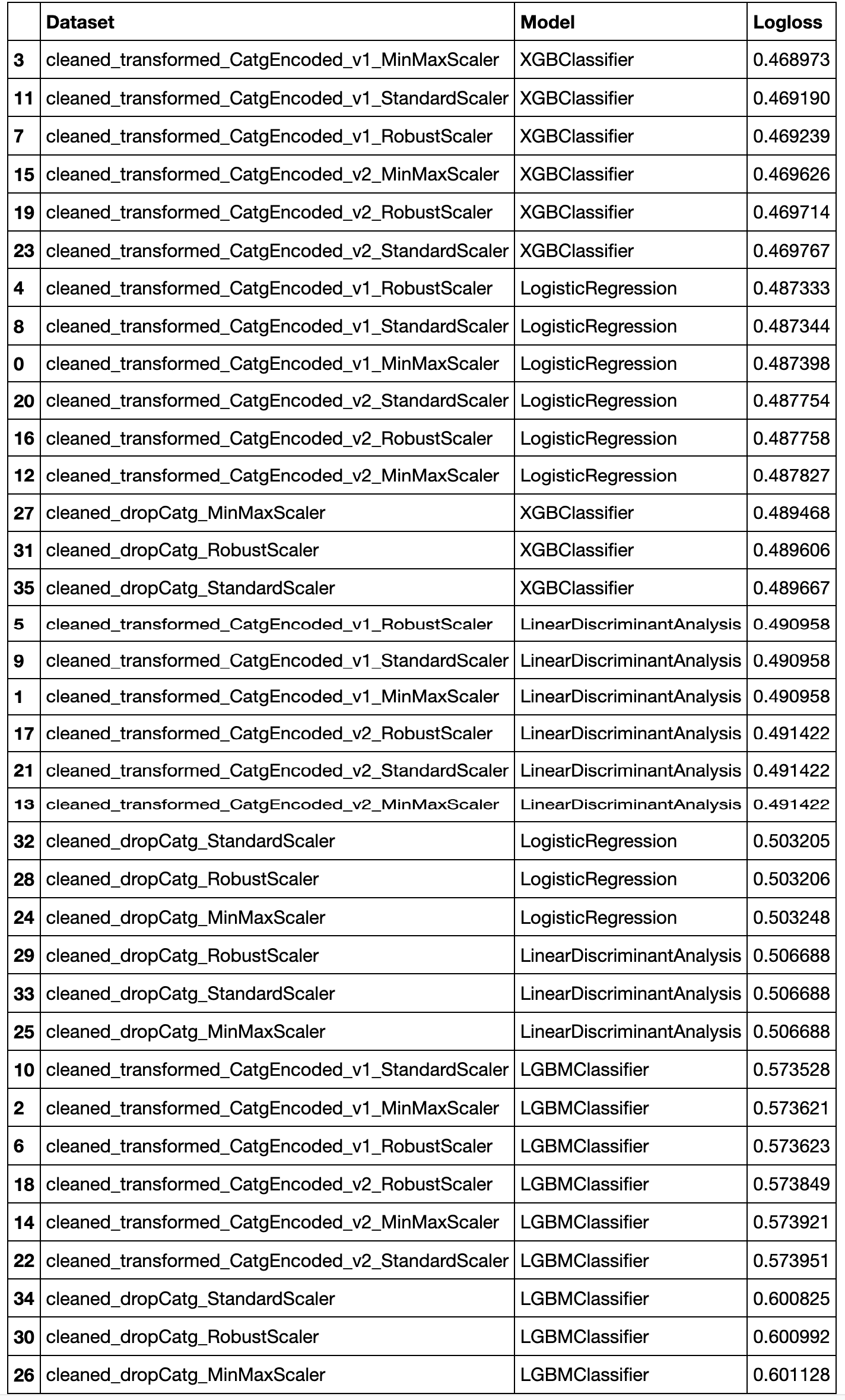
As we can see, the best is from the cleaned_transformed_CatgEncoded_v1_MinMaxScaler dataset and XGBClassifier model.

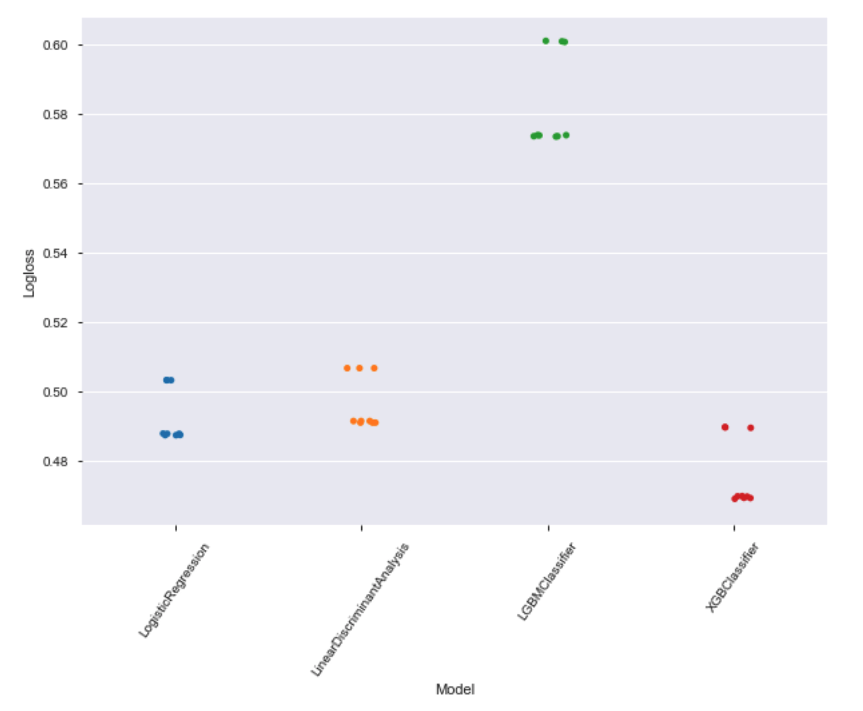
Let's see the models with the best results

#sns.stripplot(x = 'Model', y = 'Logloss', data = results, jitter = True)

plt.figure(figsize=(10,7))
chart = sns.stripplot(x = 'Model', y = 'Logloss', data = results)
chart.set_xticklabels(chart.get_xticklabels(), rotation=55)
plt.show();

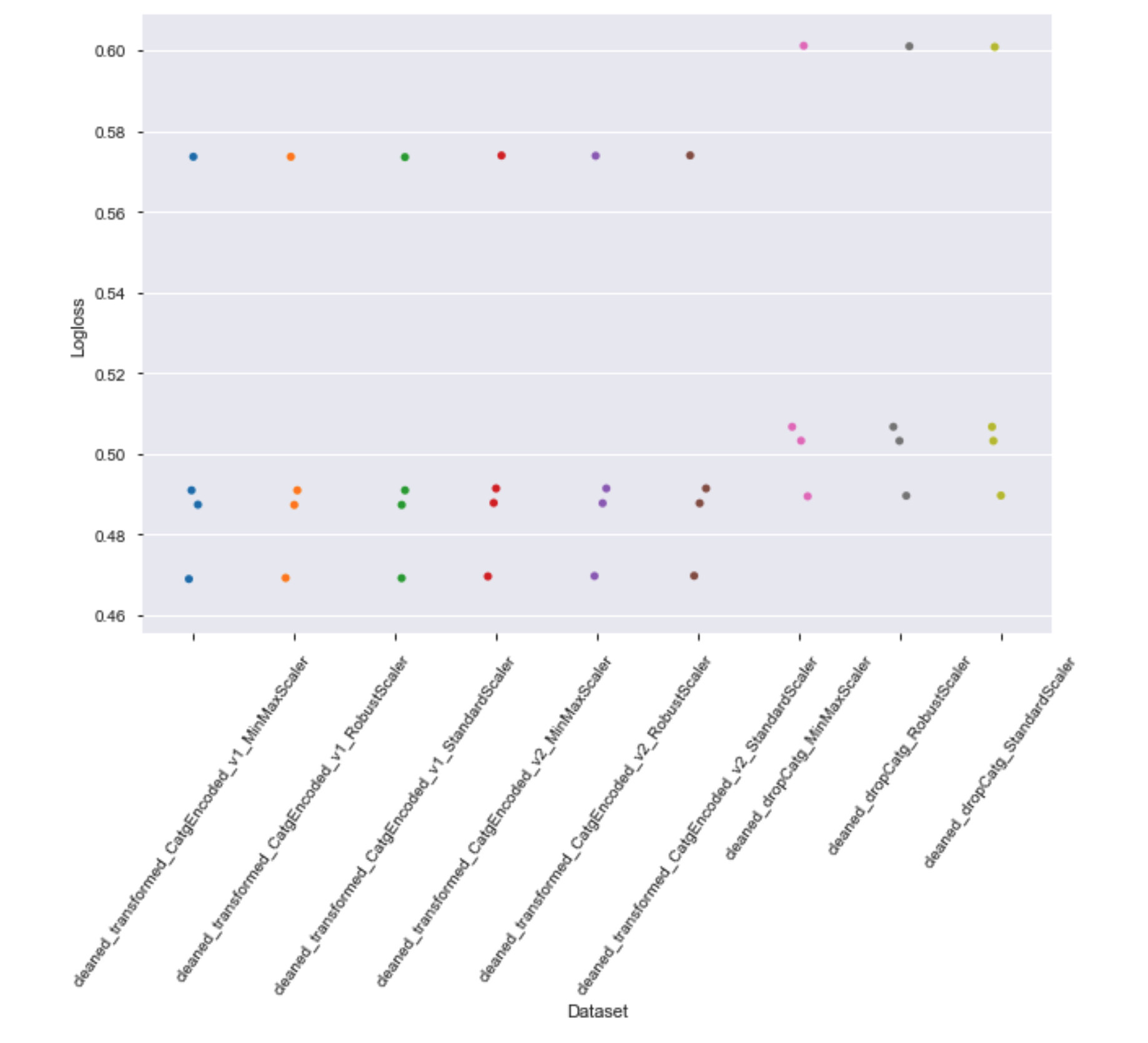
Let's check the results for each dataset:

plt.figure(figsize=(10,7))
chart = sns.stripplot(x = 'Dataset', y = 'Logloss', data = results)
chart.set_xticklabels(chart.get_xticklabels(), rotation=55)
plt.show();

Feature Selection

Our model has a lot of features, let's see the importance of each feature in the prediction process.

train = data['cleaned_transformed_CatgEncoded_v1_MinMaxScaler']['train']
train_x = train.drop(['target'], axis=1)
train_y = train['target']

# train model
best_model = XGBClassifier(learning_rate = 0.1,
                    n_estimators = 200,
                    max_depth = 5,
                    min_child_weight = 1,
                    gamma = 0,
                    subsample = 0.8,
                    colsample_bytree = 0.8,
                    objective = 'binary:logistic',
                    n_jobs = -1,
                    scale_pos_weight = 1,
                    verbose = False,
                    seed = 32)

best_model.fit(train_x, train_y, eval_metric='logloss', verbose=False )        

fig, ax = plt.subplots(figsize=(17,15))
plot_importance(best_model, ax=ax)
plt.show()

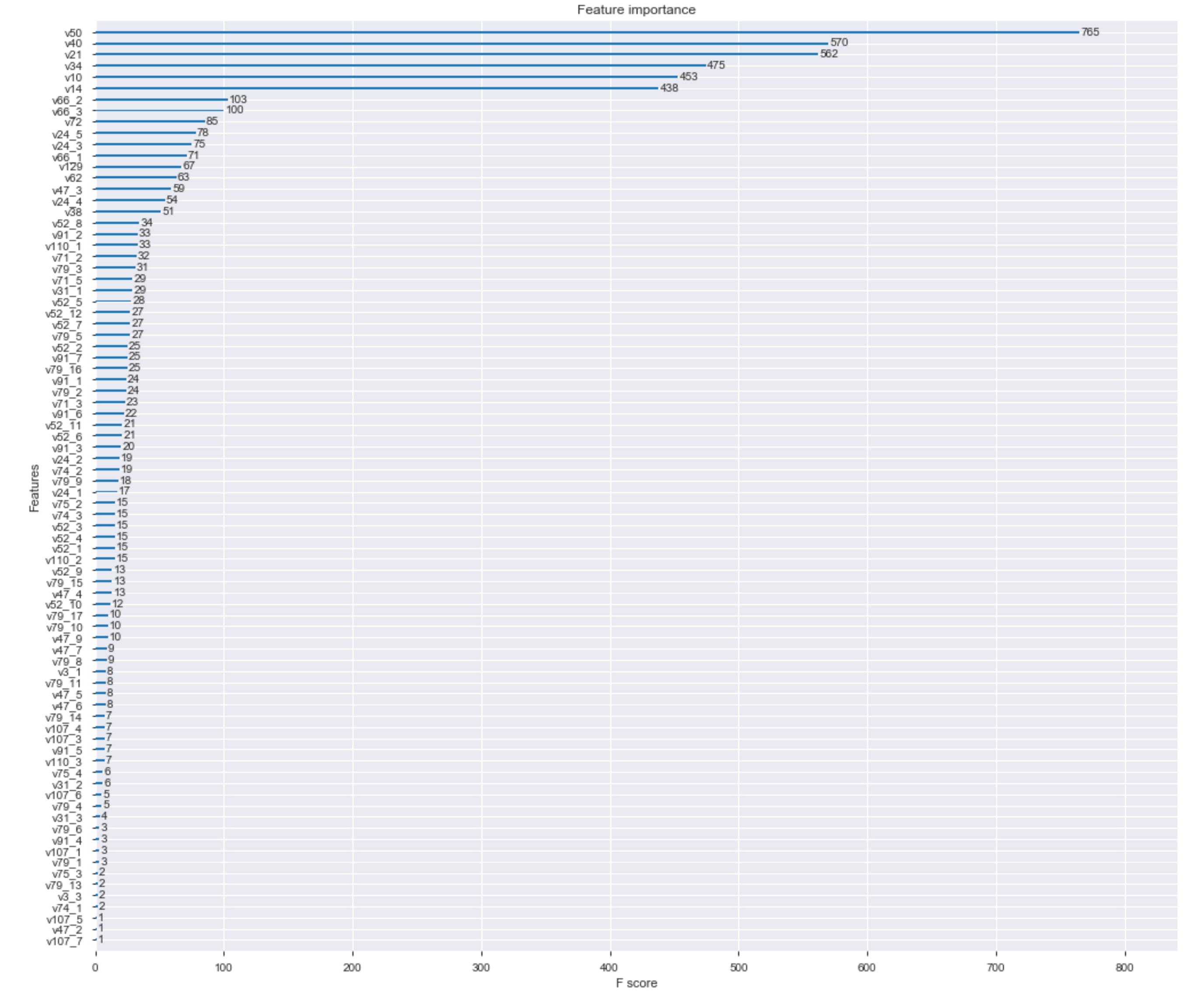
Now, that we know the importance of each feature, let's evaluate the results when removing the less important features.

# Fit model using each importance as a threshold
thresholds = sort(best_model.feature_importances_)

# Split the dataset
X_train, X_test, y_train, y_test = train_test_split(train_x, train_y, test_size=0.3, random_state=7)

# Evaluate the result for several thresholds (different number of features)
for thresh in sort(list(set(thresholds))):
    # select features using threshold
    selection = SelectFromModel(best_model, threshold=thresh, prefit=True)
    select_X_train = selection.transform(X_train)

    # train model
    selection_model = XGBClassifier(learning_rate = 0.1,
                    n_estimators = 200,
                    max_depth = 5,
                    min_child_weight = 1,
                    gamma = 0,
                    subsample = 0.8,
                    colsample_bytree = 0.8,
                    objective = 'binary:logistic',
                    n_jobs = -1,
                    scale_pos_weight = 1,
                    verbose = False,
                    seed = 32)

    selection_model.fit(select_X_train, y_train, eval_metric='logloss', verbose=False )        

    # eval model    
    select_X_test = selection.transform(X_test)
    y_pred = selection_model.predict(select_X_test)        
    train_pred_prob = selection_model.predict_proba(select_X_test)[:,1]    
    log_loss_score = log_loss(y_test, train_pred_prob)   

    print("Thresh=%.3f, n=%d, logloss: %.6f" % (thresh, select_X_train.shape[1], log_loss_score))

Thresh=0.000, n=95, logloss: 0.468835
Thresh=0.001, n=82, logloss: 0.469082
Thresh=0.002, n=81, logloss: 0.468746
Thresh=0.002, n=80, logloss: 0.469428
Thresh=0.002, n=79, logloss: 0.469242
Thresh=0.002, n=78, logloss: 0.469183
Thresh=0.003, n=77, logloss: 0.469433
Thresh=0.003, n=76, logloss: 0.469526
Thresh=0.003, n=75, logloss: 0.469013
Thresh=0.003, n=74, logloss: 0.469127
Thresh=0.003, n=73, logloss: 0.468770
Thresh=0.003, n=72, logloss: 0.468592
Thresh=0.004, n=71, logloss: 0.468956
Thresh=0.004, n=70, logloss: 0.468822
Thresh=0.004, n=69, logloss: 0.469150
Thresh=0.004, n=68, logloss: 0.469049
Thresh=0.004, n=67, logloss: 0.469318
Thresh=0.004, n=66, logloss: 0.468910
Thresh=0.004, n=65, logloss: 0.468939
Thresh=0.004, n=64, logloss: 0.469407
Thresh=0.004, n=63, logloss: 0.469481
Thresh=0.004, n=62, logloss: 0.469235
Thresh=0.004, n=61, logloss: 0.469256
Thresh=0.004, n=60, logloss: 0.469047
Thresh=0.004, n=59, logloss: 0.469205
Thresh=0.004, n=58, logloss: 0.468930
Thresh=0.004, n=57, logloss: 0.469266
Thresh=0.004, n=56, logloss: 0.469182
Thresh=0.005, n=55, logloss: 0.469258
Thresh=0.005, n=54, logloss: 0.469349
Thresh=0.005, n=53, logloss: 0.469363
Thresh=0.005, n=52, logloss: 0.469306
Thresh=0.005, n=51, logloss: 0.469264
Thresh=0.005, n=50, logloss: 0.469304
Thresh=0.005, n=49, logloss: 0.468915
Thresh=0.005, n=48, logloss: 0.468851
Thresh=0.005, n=47, logloss: 0.469583
Thresh=0.005, n=46, logloss: 0.468976
Thresh=0.005, n=45, logloss: 0.469182
Thresh=0.005, n=44, logloss: 0.469065
Thresh=0.005, n=43, logloss: 0.469279
Thresh=0.005, n=42, logloss: 0.469422
Thresh=0.005, n=41, logloss: 0.469245
Thresh=0.006, n=40, logloss: 0.469786
Thresh=0.006, n=39, logloss: 0.469703
Thresh=0.006, n=38, logloss: 0.469336
Thresh=0.006, n=37, logloss: 0.469417
Thresh=0.006, n=36, logloss: 0.469500
Thresh=0.006, n=35, logloss: 0.469238
Thresh=0.006, n=34, logloss: 0.469542
Thresh=0.006, n=33, logloss: 0.469481
Thresh=0.006, n=32, logloss: 0.469458
Thresh=0.006, n=31, logloss: 0.469541
Thresh=0.006, n=30, logloss: 0.469725
Thresh=0.006, n=29, logloss: 0.469861
Thresh=0.007, n=28, logloss: 0.469833
Thresh=0.007, n=27, logloss: 0.471707
Thresh=0.007, n=26, logloss: 0.471710
Thresh=0.007, n=25, logloss: 0.471684
Thresh=0.007, n=24, logloss: 0.472283
Thresh=0.008, n=23, logloss: 0.472345
Thresh=0.008, n=22, logloss: 0.472347
Thresh=0.008, n=21, logloss: 0.472441
Thresh=0.008, n=20, logloss: 0.472578
Thresh=0.009, n=19, logloss: 0.472788
Thresh=0.010, n=18, logloss: 0.473171
Thresh=0.010, n=17, logloss: 0.473237
Thresh=0.011, n=16, logloss: 0.473219
Thresh=0.012, n=15, logloss: 0.474140
Thresh=0.012, n=14, logloss: 0.475123
Thresh=0.013, n=13, logloss: 0.475140
Thresh=0.013, n=12, logloss: 0.475730
Thresh=0.015, n=11, logloss: 0.475717
Thresh=0.017, n=10, logloss: 0.477280
Thresh=0.019, n=9, logloss: 0.477533
Thresh=0.031, n=8, logloss: 0.477939
Thresh=0.038, n=7, logloss: 0.477914
Thresh=0.044, n=6, logloss: 0.484224
Thresh=0.046, n=5, logloss: 0.484473
Thresh=0.049, n=4, logloss: 0.516446
Thresh=0.072, n=3, logloss: 0.516690
Thresh=0.096, n=2, logloss: 0.527583
Thresh=0.178, n=1, logloss: 0.531174

As we see in the results, the removal of the lessen important features does not improve the results. Let's keep all the current features.

Imbalanced datasets

Most machine learning algorithms work better when the number of instances of each class is roughly equal.

Let's see the class distribution for the training dataset.

train = data['cleaned_transformed_CatgEncoded_v1_MinMaxScaler']['train']
print(train.target.value_counts())
train.target.value_counts().plot(kind='bar', title='Count (target)');

1    87021
0    27300
Name: target, dtype: int64

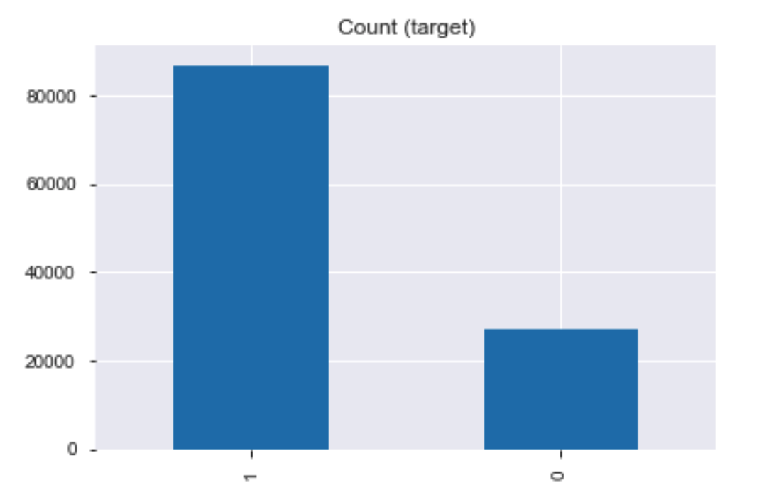
The training dataset is imbalanced.

SMOTE

Let's use the Synthetic Minority Oversampling Technique (SMOTE) to improve the class distribution.

train_x = train.drop(['target'], axis=1)
train_y = train['target']
x_train, x_val, y_train, y_val = train_test_split(train_x, train_y,
                                                  test_size = .3,
                                                  random_state=12)

sm = SMOTE(random_state=12, sampling_strategy=0.9)#{1: 10, 0: 10})
x_train_res, y_train_res = sm.fit_sample(x_train, y_train)

y_train_res.value_counts().plot(kind='bar')

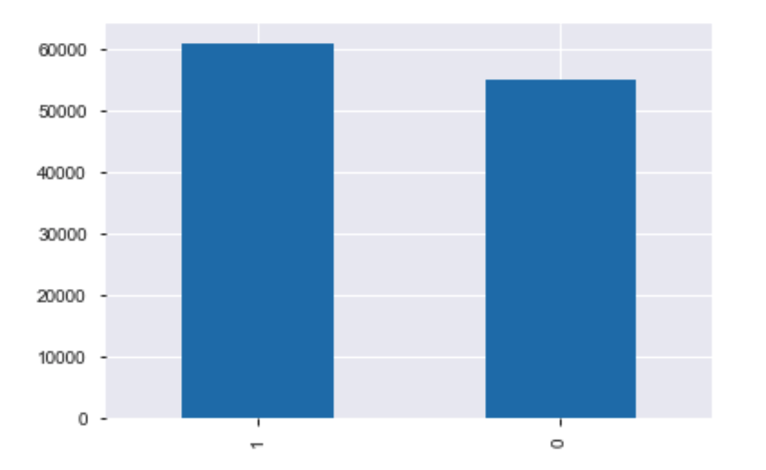
The training dataset is balanced, let's see if the results are improved.

# train model
selection_model = XGBClassifier(learning_rate = 0.1,
                    n_estimators = 200,
                    max_depth = 5,
                    min_child_weight = 1,
                    gamma = 0,
                    subsample = 0.8,
                    colsample_bytree = 0.8,
                    objective = 'binary:logistic',
                    n_jobs = -1,
                    scale_pos_weight = 1,
                    verbose = False,
                    seed = 32)

selection_model.fit(x_train_res, y_train_res, eval_metric='logloss', verbose=False )        

# eval model    
train_pred_prob = selection_model.predict_proba(x_val)[:,1]    
log_loss_score = log_loss(y_val, train_pred_prob)   
print(log_loss_score)

0.5107384842840859

There was no improvement after the use of SMOTE.

Let's keep the previous version of the dataset and generate the submission file.

Submission

Now let's build the final model using the best combination of dataset and ML algorithm and create the submission file.

# Train with the model that had the best result
selection_model = XGBClassifier(learning_rate = 0.1,
                    n_estimators = 200,
                    max_depth = 5,
                    min_child_weight = 1,
                    gamma = 0,
                    subsample = 0.8,
                    colsample_bytree = 0.8,
                    objective = 'binary:logistic',
                    n_jobs = -1,
                    scale_pos_weight = 1,
                    verbose = False,
                    seed = 32)

train = data['cleaned_transformed_CatgEncoded_v1_MinMaxScaler']['train']
train_x = train.drop(['target'], axis=1)
train_y = train['target']

final_model = selection_model.fit(train_x, train_y, eval_metric='logloss', verbose=False )        

# Test data for submission
test  = data['cleaned_transformed_CatgEncoded_v1_MinMaxScaler']['test']
test_x = test.drop(['ID'], axis=1)

# Performing predictions
test_pred_prob = final_model.predict_proba(test_x)[:,1]
submission = pd.DataFrame({'ID': test["ID"], 'PredictedProb': test_pred_prob.reshape((test_pred_prob.shape[0]))})
print(submission.head(10))

   ID  PredictedProb
0   0       0.434640
1   1       0.930129
2   2       0.868351
3   7       0.749811
4  10       0.788460
5  11       0.611152
6  13       0.956794
7  14       0.580155
8  15       0.890578
9  16       0.885386

submission.to_csv('submission.csv', index=False)

Thus, in this competition, my best score was 0.4929 and I got position 38 on the leaderboard.

Accelerating payment clearance process for an Insurance Company

Comments

My blog

Classifying the floor surface to help a robot

More from this blog

The "Vibe Coding" Revolution: Redefining Software Development in 2025

Automated Tests: The Secret to Peaceful Nights

Harness the Power of AI: How ChatGPT Can Boost Your Business Efficiency

MLOps: What it is and why does it Matter?

Basket Icon Detector

Building the prediction model

Solution

Loading the datasets

Data Cleaning

Data Analysis

Features highly correlated

Features with highly cardinality

Features with many zeros.

Feature Engineering

Enconding categorical features

Transforming numerical features

Machine Learning

Feature Selection

Imbalanced datasets

SMOTE

Submission

Command Palette

Comments

My blog

Classifying the floor surface to help a robot

More from this blog

Building the prediction model

Solution

Loading the datasets

Data Cleaning

Data Analysis

Features highly correlated

Features with highly cardinality

Features with many zeros.

Feature Engineering

Enconding categorical features

Transforming numerical features

Machine Learning

Feature Selection

Imbalanced datasets

SMOTE

Submission